In the previous days, we gradually built the foundation for understanding how speech is represented for machines.

From Waveforms to Perceptual Speech Representations

Day 1 introduced how sound becomes digital:

Air pressure vibration → microphone → sampled waveform x[n]

This waveform is simply air pressure values measured over time.

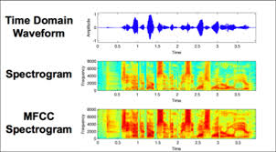
From Waveforms to Spectrograms

Day 2 showed how we analyze this waveform using the Short-Time Fourier Transform (STFT). Instead of only seeing amplitude over time, we discovered how to reveal which frequencies exist at each moment, producing the spectrogram.
X(t,f)

A spectrogram shows:

• time on the x-axis
• frequency on the y-axis
• energy as intensity

Human Perception vs Physical Frequency

Day 3 introduced an important insight:

The spectrogram describes physical sound, but human hearing does not perceive sound linearly.

So we modified the representation using:

• Mel frequency scaling (perceptual pitch spacing)
• Log compression (perceptual loudness)

This gave us the Log-Mel Spectrogram, which already resembles how the human ear organizes sound.

But in many speech systems, we go one step further.

We convert this representation into something called MFCCs (Mel-Frequency Cepstral Coefficients).

What Are MFCCs?

MFCCs are one of the most influential feature representations in speech processing. They take the spectral information of speech and compress it into a small set of numbers that capture the important characteristics of the vocal tract.

To understand why MFCCs work and how they are computed, we need to carefully walk through the entire MFCC pipeline.

Why We Need Feature Extraction

A raw waveform contains enormous detail.

For example, if speech is sampled at 16,000 Hz, that means:

1 second of audio → 16,000 samples

If we feed raw samples directly into classical machine learning systems, two problems arise:

1. Redundancy: Neighboring samples are highly correlated. Much of the information is repeated.

2. Irrelevant detail: Speech recognition does not need every microscopic vibration of air. What matters more is the shape of the frequency spectrum, which is determined by how the vocal tract filters sound.

MFCCs aim to represent exactly this.

They compress speech into a compact representation that captures the spectral envelope of the signal, which carries phonetic information.

Instead of thousands of samples per second, we may only use 13–40 coefficients per frame.

But how do we get from the waveform to those coefficients?

We do it through a sequence of carefully designed steps.

Step 1 — Pre-Emphasis

The first operation slightly amplifies high frequencies.

The pre-emphasis filter is defined as:

y[n] = x[n] - αx[n-1]

where

• x[n] is the original signal
• y[n] is the filtered signal
• α is typically around 0.95

This equation subtracts a fraction of the previous sample from the current sample.

What does this do?

This acts like a high-pass filter, which boosts higher frequencies relative to lower ones.

This step is needed because natural speech has a spectral tilt.

Due to the physics of sound production in the vocal tract:

• Low frequencies often contain much more energy
• High frequencies tend to be weaker

If we analyze speech without correcting this, the low-frequency components dominate the spectrum.

Pre-emphasis partially balances the spectrum so that higher-frequency information (which can be important for distinguishing consonants) becomes more visible.

Conceptually:

Original spectrum → dominated by low frequencies
After pre-emphasis → more balanced spectrum

This prepares the signal for better frequency analysis.

Step 2 — Framing

Speech is constantly changing.

If we analyze a long segment of speech all at once, the signal is not stationary. Its statistical properties change over time as phonemes are produced.

However, over very short intervals, speech behaves approximately stationary.

So we split the signal into small overlapping segments called frames.

Typical parameters are:

• Frame length: 20–25 milliseconds
• Frame step: 10 milliseconds

For example:

|-----25ms-----|
      |-----25ms-----|
            |-----25ms-----|

Each frame overlaps slightly with the next one.

Why overlap?

Because speech transitions smoothly. Overlapping frames ensure we do not lose important information between boundaries.

Each frame is analyzed independently.

Step 3 — Windowing

When we cut a frame from the waveform, we introduce sharp edges at the boundaries.

These abrupt edges create artificial frequency components when we perform a Fourier transform. This phenomenon is called spectral leakage.

To reduce this problem, we multiply each frame by a window function.

The most common window used in speech processing is the Hamming window.

w[n] = 0.54 - 0.46cos(2πn/N-1)

The window gradually reduces the amplitude near the edges of the frame.

Instead of abruptly cutting the signal, the window gently tapers it toward zero.

So the frame transitions smoothly from zero → full amplitude → zero.

This reduces artificial frequencies in the spectral analysis.

Step 4 — Fourier Transform (FFT)

Now we analyze the frequency content of each frame.

We apply the Fast Fourier Transform (FFT), which efficiently computes the Discrete Fourier Transform.

X[k]=n=0∑N−1​x[n]e−j2πkn/N

This transformation converts the signal from the time domain into the frequency domain.

The result tells us:

• which frequencies are present
• how strong each frequency is

Usually we compute the power spectrum:

P[k] = |X[k]|^2

This gives the energy present at each frequency.

At this point we have a spectrum for each frame.

However, the frequencies are still linearly spaced in Hertz, which does not reflect how humans perceive pitch.

Step 5 — Mel Filterbank

This is where we reconnect with Day 3.

Human pitch perception is not linear.

The difference between 200 Hz and 300 Hz feels much larger than the difference between 5200 Hz and 5300 Hz, even though both differences are 100 Hz.

This happens because the ear’s frequency resolution is approximately logarithmic.

To reflect this, we transform the frequency axis into the Mel scale, which approximates perceived pitch.

The Mel scale is defined as:

Mel(f) = 2595 log10(1 + f/700)

Using this scale, we create a bank of triangular filters spaced evenly in Mel units.

Each filter captures energy from a small frequency region.

The energy in the (m)-th Mel band is computed as:

Mm = ∑ P[k]Hm[k]
k

where Hm[k] is the (m)-th filter.

Instead of hundreds of FFT frequency bins, we now obtain around 20–40 Mel band energies.

This step performs two things:

1. Reduces dimensionality
2. Aligns frequency analysis with human hearing

Step 6 — Logarithmic Compression

Next we apply a logarithm to each Mel band energy:

Lm​=log(Mm​)

This step is motivated by how humans perceive loudness.

The ear does not perceive loudness linearly.

Instead, loudness perception roughly follows a logarithmic relationship with physical sound intensity.

For example:

• Increasing sound power by 10× does not feel 10× louder.

The log operation also compresses the dynamic range of the signal, making features more stable and easier for models to learn from.

At this stage we have the Log-Mel spectrum.

Step 7 — Discrete Cosine Transform (DCT)

The final step converts the Log-Mel spectrum into MFCC coefficients.

Adjacent Mel bands are strongly correlated because the spectrum changes smoothly.

The Discrete Cosine Transform (DCT) decorrelates these values.

cn​=m=1∑M​Lm​cos(Mπn​(m−0.5))

The DCT transforms the spectral information into a new space where:

• most information is concentrated in the first few coefficients
• higher coefficients contain finer details

Usually we keep only 12–13 coefficients.

These numbers are the Mel-Frequency Cepstral Coefficients.

The Complete MFCC Pipeline

If we connect all the steps, the transformation looks like this:

Raw waveform
      ↓
Pre-emphasis
      ↓
Framing
      ↓
Windowing
      ↓
FFT → Power Spectrum
      ↓
Mel Filterbank
      ↓
Log Compression
      ↓
Discrete Cosine Transform
      ↓
MFCC Feature Vector

Each frame of speech becomes a small vector such as:

[c1, c2, c3, ..., c13]

These vectors are what classical speech recognition systems use as input.

Why MFCCs Are So Effective

Speech sounds are produced when the vocal cords generate a sound source, which is then filtered by the shape of the vocal tract.

The resulting sound contains a spectral envelope that reflects the configuration of the mouth, tongue, and throat.

MFCCs are designed specifically to capture this envelope while ignoring irrelevant details like pitch harmonics.

Because of this, MFCCs became a standard feature representation in:

• Automatic Speech Recognition (ASR)
• Speaker Identification
• Emotion Detection
• Language Identification

Even many modern deep learning systems still use Log-Mel or MFCC features as their input representation.

Final Intuition

Think of the MFCC pipeline as a series of transformations that move from raw physics to perceptual abstraction.

First we observe the physical signal.

Then we reshape it according to how humans hear.

Finally, we compress it into a compact numerical description of speech structure.

In other words:

Air vibration
     ↓
Waveform
     ↓
Spectral analysis
     ↓
Perceptual frequency scaling
     ↓
Compact speech features

MFCCs are essentially a mathematical approximation of the early auditory processing performed by the human ear.