Imagine you're trying to teach a computer to understand speech. You could start by giving it a microphone and recording sound waves, raw numbers representing air pressure changes over time. But here's the challenge: how do you transform these numbers into something that captures what human listeners actually hear?
Yesterday, we took our first step. We transformed a waveform into a spectrogram, a visual representation showing time on one axis, frequency on another, and amplitude as brightness. Mathematically, we computed the Short Time Fourier Transform (STFT): X(t,f) = STFT{x[n]}, looking at the squared magnitude |X(t,f)|².
But this spectrogram gives us what we might call a "physical" view of sound. It's accurate in an objective sense, it faithfully records what frequencies existed when and how intense they were. However, it doesn't yet reflect how humans actually perceive sound.
Think of it this way: a raw spectrogram is like a photograph of a forest. The camera captures every leaf, every shadow, every detail with equal precision. But when a human looks at that forest, their perception isn't uniform, they notice movement, familiar shapes, contrasts that matter. Our visual system emphasizes what's important for survival and meaning.
Similarly, our auditory system doesn't treat all frequencies and amplitudes equally. We need to modify our sound representation so that it reflects what humans actually hear, the differences that matter for communication, emotion, and meaning.
A standard STFT spectrogram makes two key assumptions that don't match human hearing.
First, it assumes linear frequency spacing. Every 100 Hz step is treated as equally important. A jump from 200 Hz to 300 Hz gets the same representation as a jump from 5200 Hz to 5300 Hz.
But here's the problem: to human ears, these jumps feel completely different. The 200 to 300 Hz shift is a noticeable pitch change, it might be the difference between two musical notes or two tones in a tonal language. The 5200 to 5300 Hz shift? Most listeners would struggle to hear any difference at all. It might as well be the same sound.
Second, it assumes linear amplitude. If a sound becomes twice as intense physically, the spectrogram shows it as twice as bright. But human loudness perception doesn't work this way. A sound that's ten times more intense physically doesn't feel ten times louder, it might feel only about twice as loud.
This creates a practical problem: a whisper and a shout might have enormously different physical energies, but our perception compresses that difference. We can hear both clearly, just as different levels of loudness within a manageable range.
For AI systems trying to learn from sound, these mismatches matter. A model trained on raw spectrograms might learn to pay too much attention to high frequency details that humans barely notice, while missing subtle but important low frequency variations. This is especially critical for tonal languages like Yoruba, Igbo, or Hausa, where pitch distinctions at lower frequencies carry meaning.
To build better representations, we need to understand the biology of hearing. Inside your ear lies the cochlea, a spiral shaped, fluid filled structure. Running along its length is the basilar membrane, which responds to sound vibrations differently depending on where you look.
Near the base, the stiff, narrow end, the membrane responds best to high frequencies. Near the apex, the wider, more flexible end, it responds best to low frequencies.
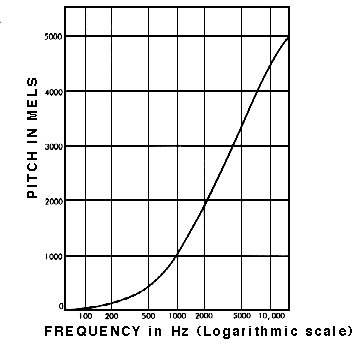
Here's the crucial insight: this mapping from frequency to position along the membrane isn't linear. It's roughly logarithmic. Equal steps in perceived pitch correspond to multiplicative steps in physical frequency.
This means humans perceive ratios of frequencies, not absolute differences. When you double a frequency, say from 200 Hz to 400 Hz, you hear a specific musical interval, an octave. That same ratio feels similar whether you're going from 200 Hz to 400 Hz or from 2000 Hz to 4000 Hz. But the absolute difference? 200 Hz versus 400 Hz is very different from 2000 Hz versus 4000 Hz in terms of perceived pitch change.
This logarithmic perception explains why our earlier example matters. 200 to 300 Hz represents a 1.5 times ratio, a noticeable musical fifth. 5200 to 5300 Hz represents only a 1.02 times ratio, barely a blip in pitch space.
To model this perceptual reality, researchers developed the Mel scale, a mapping from physical frequency measured in Hertz to perceived pitch measured in mels. The name comes from "melody," reflecting its musical motivation.
The standard formula is:
Mel(f) = 2595 × log₁₀(1 + f/700)
Let's unpack what this does.
Below about 1000 Hz, the mapping is nearly linear. A change of 100 Hz here feels like a real pitch difference. Above 1000 Hz, the mapping becomes increasingly logarithmic. Higher frequencies get "compressed," a 100 Hz change at high frequencies represents a much smaller perceptual change.
This transformation accomplishes something essential: it preserves detail where human hearing is most sensitive, the low frequencies that carry speech prosody, tone, and musical bass, and compresses information where human perception is less discriminating, high frequencies where we mainly detect presence rather than precise pitch.
For speech AI, this means our models will focus their representational capacity on the frequency ranges that matter most for human communication.
Now we can combine our STFT spectrogram with the Mel scale to create something more perceptually relevant. Here's how it works.
Step 1: Start with the STFT. We compute the spectrogram as before, giving us energy at each time and each linear frequency bin.
Step 2: Design a Mel filterbank. We create a set of triangular filters, each centered at a specific Mel scale frequency. These filters are evenly spaced along the Mel scale, meaning they get wider in Hertz as frequency increases, and they overlap, mimicking how auditory filters overlap in the cochlea.
Step 3: Apply the filters. For each time frame, we multiply the STFT magnitude by each Mel filter and sum the results. Mathematically:
M(t,m) = ∑|X(t,f)|² × Hₘ(f)
where Hₘ(f) is the mth Mel filter.
The result is a new representation: time on one axis, Mel channels on the other, with values representing the energy in each perceptual frequency band.
Notice what's happened. Low frequencies now have narrow, closely spaced bands, giving good detail. High frequencies have wide, sparse bands, giving less detail, matching perception.
We've fixed frequency, but amplitude is still linear. A sound with twice the physical energy still shows up as twice the value in our Mel spectrogram. Human hearing, however, compresses this range dramatically.
Consider that human hearing spans about 120 decibels, that's a trillion fold range in intensity, ten to the power of twelve. We can hear a pin drop and a jet engine, but our perception of loudness doesn't track this enormous physical range linearly. Instead, we perceive loudness roughly logarithmically. Each doubling of perceived loudness requires about a tenfold increase in physical intensity.
To model this, we apply logarithmic compression:
S(t,m) = log(M(t,m) + ε)
The small constant ε prevents taking the log of zero, which would be undefined. This simple transformation makes soft sounds more visible in the representation, compresses the enormous range of loud sounds, and creates a representation where differences more closely match perceived loudness differences.
Now we have it, the Log Mel spectrogram, a representation that reflects both pitch perception through Mel scaling and loudness perception through log compression.
Before we finish, let's briefly touch on a related concept: the Bark scale. While the Mel scale models pitch perception, how far apart frequencies feel, the Bark scale models something different, auditory filtering and masking.
The ear acts like a set of about 24 overlapping bandpass filters, called critical bands. Frequencies that fall within the same critical band can mask each other. A louder sound can make a quieter sound at a nearby frequency completely inaudible.
The Bark scale maps physical frequency to these perceptual bands. It's coarser than the Mel scale in some ways, but it captures important interactions between frequencies.
Both scales help us approximate the front end processing of human hearing. The Mel scale tells us about resolution. The Bark scale tells us about interference. For many speech applications, the Mel scale, especially with log compression, provides an excellent balance of perceptual relevance and computational practicality.
Let's trace our journey through representations.
| Step | Representation | What It Captures |
|---|---|---|
| Day 1 | x[n] waveform | Raw amplitude over time, the physical pressure changes reaching the microphone |
| Day 2 | X(t,f) STFT | Physical frequency content over time, linear axes, objective but not perceptual |
| Day 3 | M(t,m) to S(t,m) Log Mel | Perceptual frequency bands with logarithmic loudness, what humans actually hear |
Each transformation brings us closer to modeling sound the way human listeners experience it. The waveform is pure physics. The STFT adds frequency decomposition but remains linear. The Log Mel spectrogram finally incorporates the nonlinearities of human perception.
This isn't just academic curiosity. It has practical consequences for building better speech systems.
Improved learning efficiency. When input representations match what humans find important, neural networks can learn more effectively from less data. They don't waste capacity modeling irrelevant variations.
Preservation of tonal cues. For African languages like Yoruba, Igbo, and Hausa, tone carries meaning. The same sequence of consonants and vowels can mean different things depending on pitch patterns. By preserving low frequency detail through Mel scaling, we ensure these critical cues remain accessible to the model.
Robustness to irrelevant variation. Two different speakers might produce the same vowel with slightly different high frequency characteristics due to vocal tract differences. By compressing high frequencies, we reduce these speaker specific variations while preserving the linguistically relevant information.
Better alignment with human evaluation. Ultimately, speech systems are evaluated by how well they serve human listeners. Aligning internal representations with human perception tends to produce outputs that sound more natural and intelligible.
Here's a simple way to think about what we've accomplished.
The STFT spectrogram answers the question: what frequencies exist physically at each moment, and how intense are they?
The Mel plus Log spectrogram answers the question: what frequencies and loudness differences actually matter to human listeners, given how our ears and brains process sound?
Speech AI isn't just signal processing. It's about modeling sound the way humans hear it. By building perceptual principles into our representations, we ensure that our AI systems can learn the patterns that matter for communication: the subtle pitch movements that carry meaning in tonal languages, the relative loudness patterns that signal emphasis and emotion, and the spectral shapes that distinguish one speech sound from another.