ENCODER DECODER ACRCHITECTURE

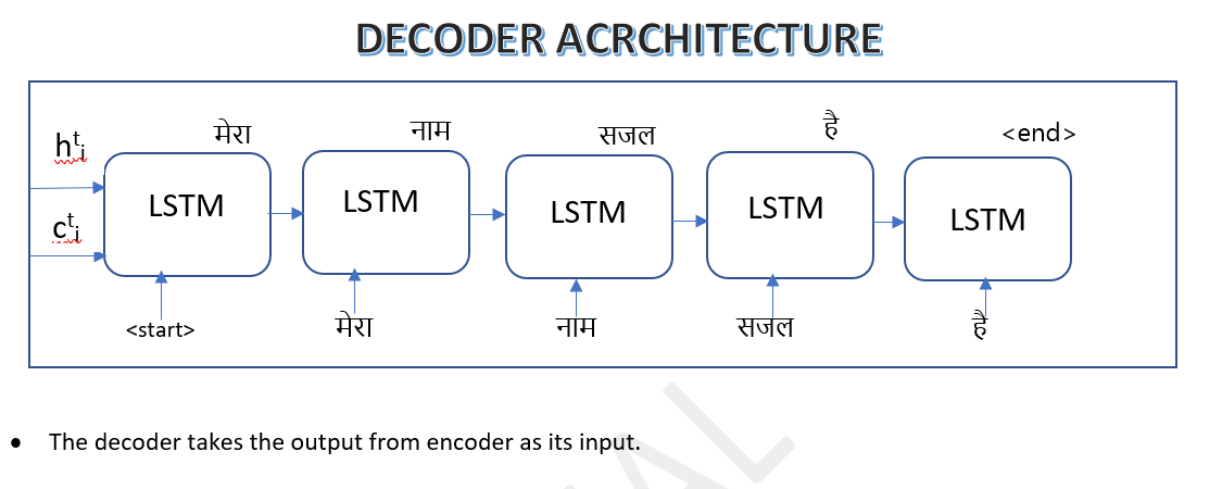
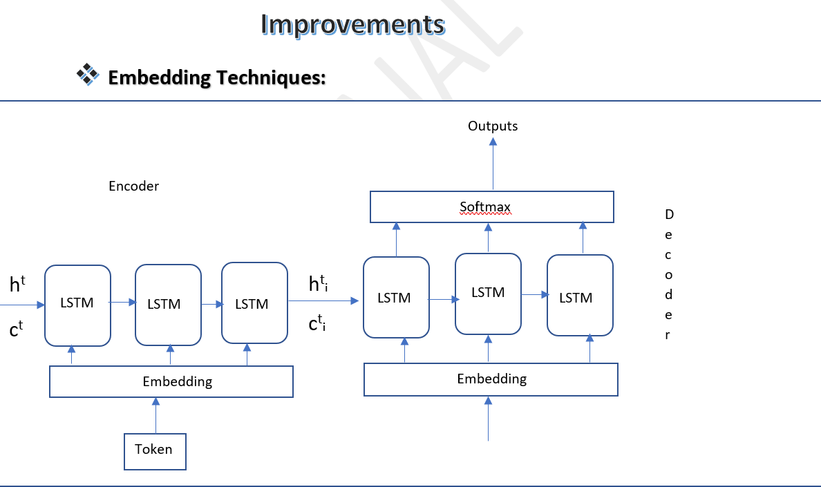
• A context vector is essentially a summary of the input data. When dealing with text, the input is typically processed token by token, where each token represents a word or a character. The goal is to convert this tokenized input into a numerical format that can be understood by machine learning models. This numerical format is known as a context vector, which is a set of numbers that encapsulate the meaning and context of the input text.

• We sent my input as a token by token to the encoder and after summatrization it gives a output in numerical format or vector format, which called vector summarization. [Vector means set of numbers].

• For summazrization purpose we basically use LSTM or some of the cases GRU(Gated Recurrent Unit).
GRU is more faster and it takes less memory than LSTM . But in Dataset LSTM is more accurate.

                    ENCODER ACRCHITECTURE

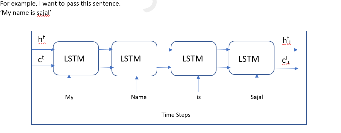
• In LSTM the cell state(ct) represent the memory of the network, storing information overtime.
• Where The hidden state(ht) in LSTM contains information that is used for the next time step. It is a more filtered version of the cell state, focusing on the information that is immediately relevant for the current time step's output and for propagating to the next time step.

                                        Training Process

Dataset
English Hindi
My name is Sajal मेरा नाम सजल है
Steps for Training

1. Forward Propagation
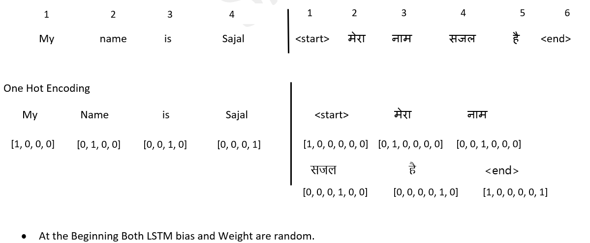
   o Convert the sentence into tokens.
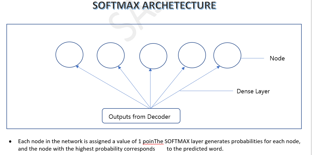
   o Convert the tokens into numerical format using one-hot encoding.
   o Pass the encoded tokens through the neural network to compute the output.
2. Calculate Loss
   o Compare the predicted output with the actual output.
   o Use a loss function (e.g., cross-entropy loss) to measure the difference.
3. Backward Propagation
   o Perform backpropagation to compute gradients.
   o Update the network parameters using an optimization algorithm (e.g., stochastic gradient descent).

1st Step is Forward Propogation

                     1st Step is Forward Propogation

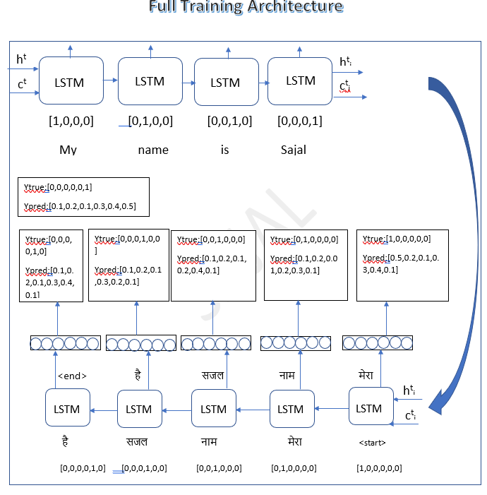
Example Scenario
Consider a scenario where we are predicting a sequence of words. At each time step, the model predicts the next word in the sequence based on the current input and the context it has learned so far. For instance, if at the second time step, the model should predict the word "नाम" but instead predicts "सजल", it indicates a deviation from the expected output.

The Challenge
According to the rules of sequence prediction, the output from the previous time step is used as the input for the current time step. In our example, even though the correct output should have been "नाम", the model's prediction "सजल" is fed into the next step. This can propagate errors and lead to incorrect predictions in subsequent steps.

Teacher Forcing
To address this issue, a technique called Teacher Forcing is employed. Teacher Forcing involves using the actual target output from the training dataset as the input for the next time step, rather than the model's predicted output. This helps the model learn the correct sequence and improves its ability to make accurate predictions.

1. Without Teacher Forcing:
   o Time Step 1 Output: "मेरा"
   o Time Step 2 Input: "मेरा"
   o Time Step 2 Output: "सजल" (incorrect)
   o Time Step 3 Input: "सजल"

2. With Teacher Forcing:
   o Time Step 1 Output: "मेरा"
   o Time Step 2 Input: "मेरा"
   o Time Step 2 Output: "सजल" (incorrect)
   o Time Step 3 Input: "नाम" (correct, from the dataset)

By using the correct input "नाम" at time step 3, as specified in the training data, the model is guided to learn the correct sequence.

                       2nd Step is Calculating Loss

After Forward Propogation Calcualte the loss
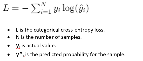
Here we are using categorical cross entropy because multiple outputs I have to choose one.
Formula for calculating loss:

               3rd Step is Gradient and Updating Parameter

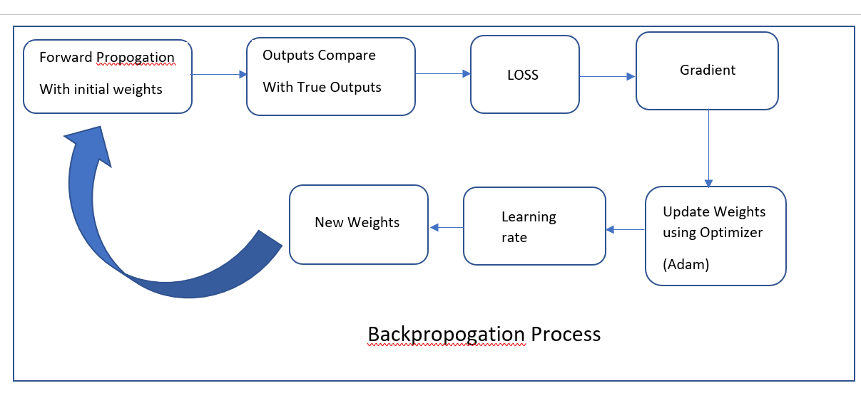
Here we calculate the loss of gradient in every trainable parameter.

Gradient Calculation and Weight Update in Neural Networks
Gradient Calculation
Gradients in neural networks quantify how each parameter (like weights and biases) affects the overall loss function. They indicate both the direction and magnitude of adjustments needed to minimize the loss during training.
• Importance: Gradients guide the optimization process by showing how parameters influence the loss.

Weight Update
Once gradients are computed, they are used to update the weights of the neural network. This process is crucial for improving model performance over iterations.
• Stochastic Gradient Descent (SGD):
o Update Rule: Adjusts weights in the direction opposite to the gradient, scaled by a learning rate.
o Purpose: Efficiently minimizes the loss by iteratively updating parameters.
• Adam Optimizer:
o Features: Integrates adaptive learning rates and bias correction.
o Advantages: Enhances convergence speed and stability across different types of datasets and models

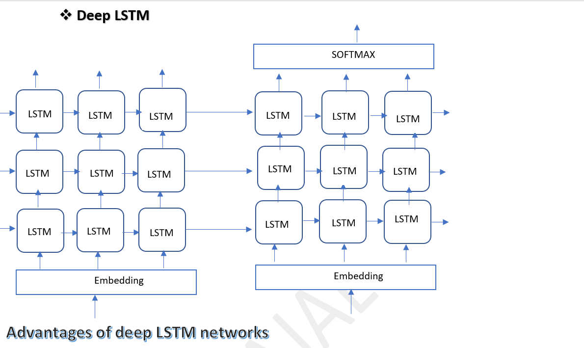
                  Advantages of deep LSTM networks

Capturing Long-Term Dependencies
• Example: Natural Language Processing (NLP)
o Scenario: Predicting the next word in a sentence requires understanding context over long sequences.
o Explanation: Deep LSTM networks effectively capture dependencies like in the sentence "The cat sat on the mat," understanding the relationship between "sat" and "mat" requires remembering the context from "The cat sat on the".

Modeling Temporal Patterns
• Example: Stock Market Prediction
o Scenario: Predicting future stock prices based on historical data with complex temporal dependencies.
o Explanation: Deep LSTM networks excel in capturing subtle changes and dependencies in stock price movements, automatically extracting features such as trends and seasonality.

Hierarchical Representation Learning
• Example: Image Captioning
o Scenario: Generating descriptive captions for images requires understanding visual content and context.
o Explanation: Deep LSTM networks learn hierarchical visual features, allowing them to generate captions like "A cat sitting on a mat" by associating visual elements with linguistic patterns.

Temporal Modeling for Speech Recognition
• Example: Speech Recognition
o Scenario: Converting spoken language into text involves understanding dynamic speech signals.
o Explanation: Deep LSTM networks model temporal dependencies in speech signals, improving accuracy by mapping acoustic features to linguistic units like phonemes and words.