TL;DR: Distance Profile is a versatile and powerful technique in time series analysis. In this work, we apply it to a task we define as Time-Step Classification, where the goal is to classify individual time steps within a time series. Our approach demonstrates its effectiveness and potential for broader applications in this domain.

Abstract

Time series analysis often requires classifying individual time points, a task we term Time-Step Classification. This publication explores the application of Distance Profile, an existing versatile technique in time series analysis, to this challenge. We adapt the Distance Profile method, using MASS (Mueen's Algorithm for Similarity Search) for efficient computation, specifically for Time-Step Classification. Our approach leverages the intuitive concept of nearest neighbor search to classify each time step based on similar sequences. We present our implementation, including modifications for multivariate time series, and demonstrate its effectiveness through experiments on diverse datasets. While not achieving the highest accuracy compared to complex models like LightGBM, this adapted method proves valuable as a strong baseline and quick prototyping tool. This work aims to highlight Distance Profile as a simple yet versatile approach for Time-Step Classification, encouraging its broader adoption in practical time series analysis.

Introduction

Time series data is ubiquitous, from stock prices to sensor readings, but analyzing it presents unique challenges. One such challenge is Time-Step Classification - labeling each point in a time series. While many complex methods exist, sometimes the most intuitive approaches yield impressive results.

In this paper, we explore Distance Profile, a method rooted in the simple concept of nearest neighbor search. We show how this straightforward idea becomes a powerful tool for Time-Step Classification:

1. We introduce Distance Profile and its applications in time series analysis.
2. We detail our implementation using the MASS algorithm, including adaptations for multivariate time series.
3. We demonstrate its effectiveness through experiments on various datasets.

By showcasing how this simple, intuitive method can tackle complex time series challenges, we aim to highlight its value for establishing baselines and quick prototyping. Our work serves as a practical guide, encouraging practitioners to consider Distance Profile alongside more advanced techniques in their analytical toolkit.

Distance Profile

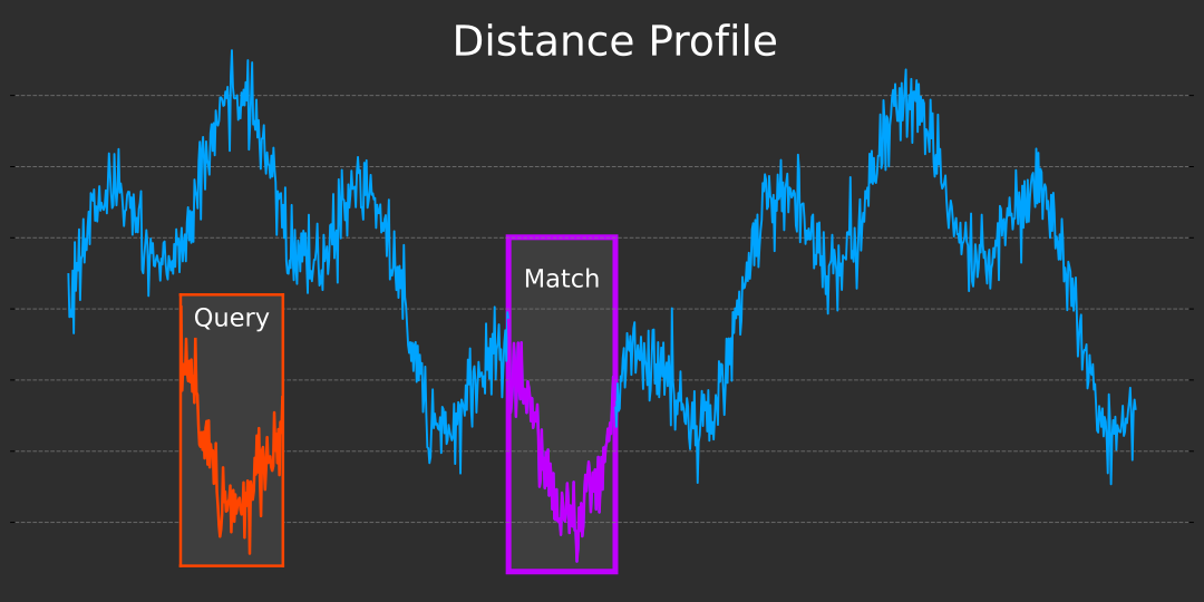
Distance Profile is a fundamental technique in time series analysis that measures the similarity between a query subsequence and all possible subsequences of a longer time series. This method is crucial for various tasks such as pattern recognition, anomaly detection, and classification in time series data.

Definition

The distance profile of a query subsequence with respect to a time series is a vector where each element represents the distance between and a corresponding subsequence of . Formally:

• Let be a time series of length .
• Let be a query subsequence of length .
• The distance profile is an length vector.
• Each element represents the distance between and the subsequence of starting at index .

Computation

The most commonly used distance measure for calculating the distance profile is the z-normalized Euclidean distance, which is robust against variations in scale and offset. The computation involves two key steps:

1. Z-Normalization: Each subsequence of the time series and the query is individually normalized to have zero mean and unit variance.
   
2. Distance Computation: The Euclidean distance between the normalized and each normalized subsequence of is calculated and stored in the distance profile vector.
   

Distance Profile Example

Sample Dataset for Demonstration
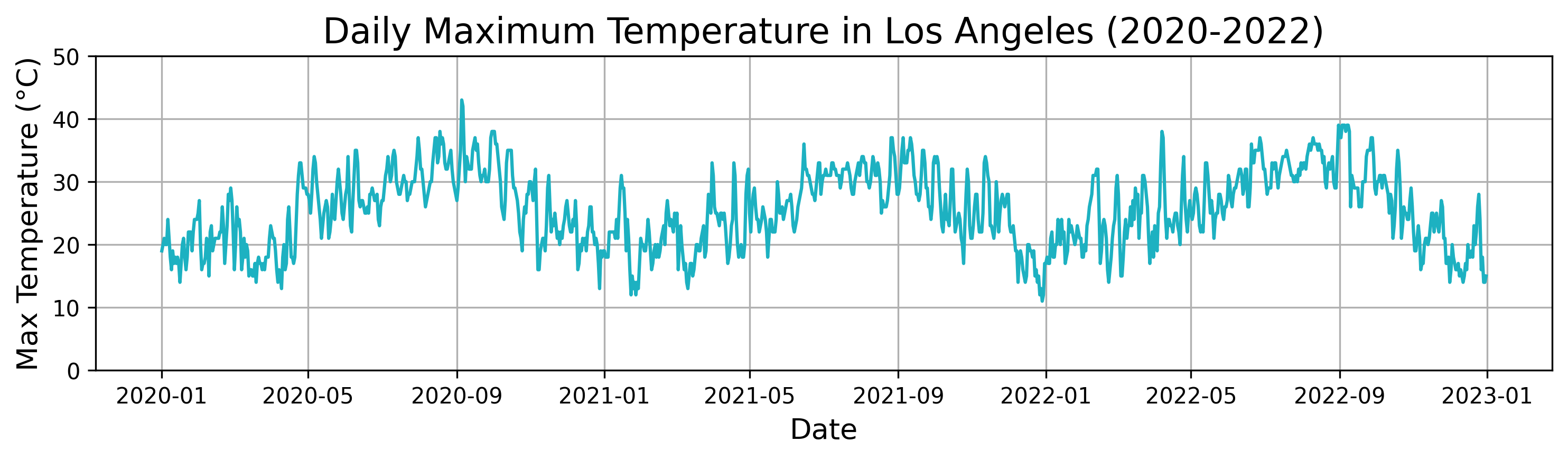
To illustrate the application of Distance Profile in Time-Step Classification, we will use a real-world time series representing daily weather data for the city of Los Angeles. This dataset spans three full years, from 2020 to 2022, and includes various meteorological parameters such as temperature, humidity, and wind speed.

We chose this dataset for its accessibility and clear seasonal patterns, making it ideal for demonstrating how Distance Profile identifies similar patterns across different time periods. Later in the experiments section, we will work with more typical, complex datasets to thoroughly evaluate the method's performance.

The dataset is uploaded in the Resources section of this article. See file titled los_angeles_weather.csv. We will use the feature series titled maxTemp for our demonstration.

Below is the plot of the daily maximum temperature in Los Angeles over the three years. It illustrates the distinct temperature patterns and seasonal fluctuations in the city, providing a rich dataset for analyzing time-series patterns.

Query Subsequence
The dataset provides an excellent example for demonstrating how Distance Profile can identify similar patterns within a time series. For our demonstration, we select a query period representing the first 10 days in the dataset (i.e., starting on January 1st and ending on January 10th, 2020.) The following chart shows the maximum temperatures over the query period.

The following chart shows the maximum temperatures over the query period.

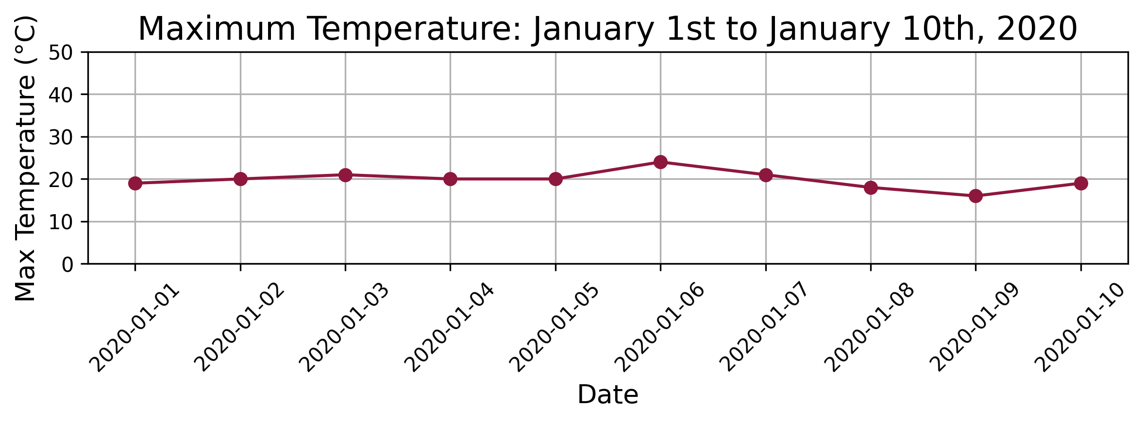
The goal of this example is to identify other similar temperature patterns throughout the three-year period using Distance Profile. By applying Distance Profile to this query subsequence, we can explore how well the technique can locate similar temperature trends within the broader time series. This exercise not only showcases the practical utility of Distance Profile but also demonstrates its effectiveness in identifying meaningful patterns in real-world weather data.

Implementation using NumPy
The following code is a simple implementation of the distance profile algorithm on a one-dimensional series.

import numpy as np

def z_normalize(ts):
    """Z-normalize a time series."""
    return (ts - np.mean(ts)) / np.std(ts)

def sliding_window_view(arr, window_size):
    """Generate a sliding window view of the array."""
    return np.lib.stride_tricks.sliding_window_view(arr, window_size)

def distance_profile(query, ts):
    """Compute the distance profile of a query within a time series."""
    query_len = len(query)
    ts_len = len(ts)

    # Z-normalize the query
    query = z_normalize(query)

    # Generate all subsequences of the time series
    subsequences = sliding_window_view(ts, query_len)

    # Z-normalize the subsequences individually
    subsequences = np.apply_along_axis(z_normalize, 1, subsequences)

    # Compute the distance profile
    distances = np.linalg.norm(subsequences - query, axis=1)

    return distances

# You can now apply the above functions to your temperature data
# by passing the relevant query and time series arrays.

# Compute the distance profile
dist_profile = distance_profile(query, time_series)

import stumpy

# ... read your data and create the query and time_series numpy arrays
# query is a 1d numpy array
# time_series is a 1d numpy array

distance_profile = stumpy.core.mass(query, time_series)

The following chart displays the distance profile for the given query and time_series. The 3 nearest-neighbors are time-windows starting on May 29th, 2020, December 3rd, 2020, and May 30th, 2021. These are the locations in the time series where the distance profile values are the lowest, indicating the most similar subsequences to the query.

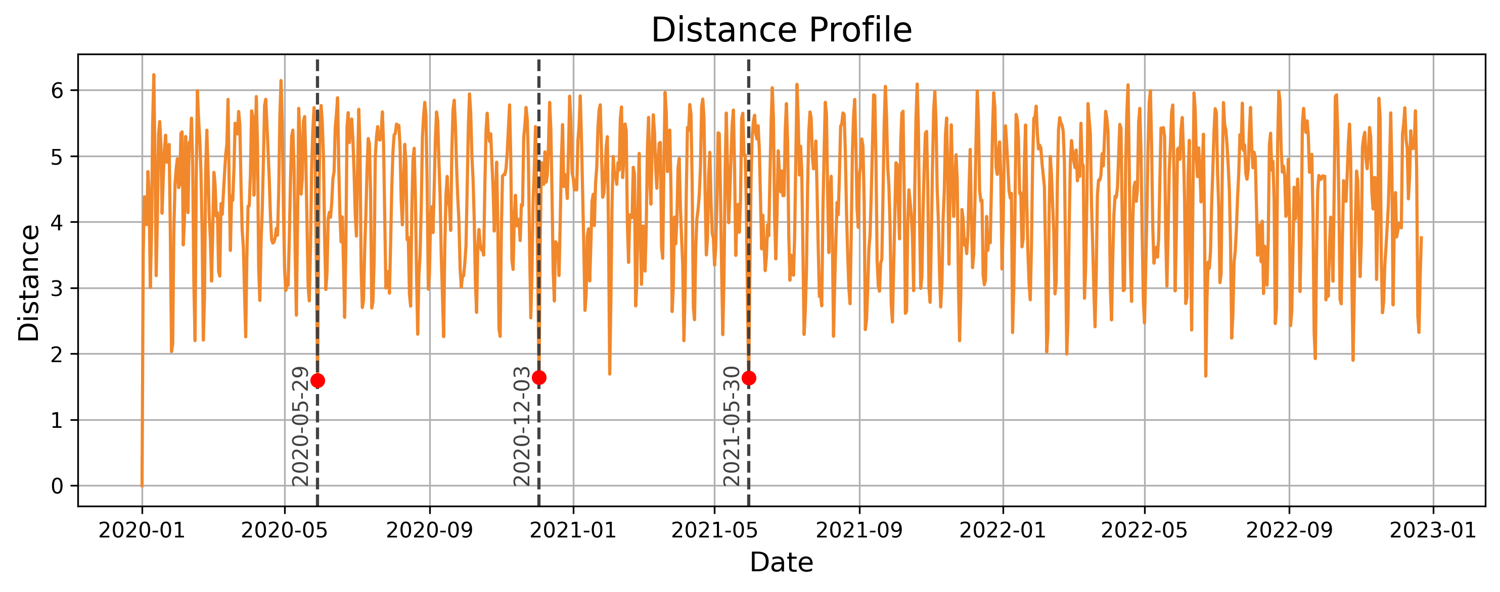
Next, we visualize and compare the patterns in the 3 nearest neighbors with the original query in the following chart.

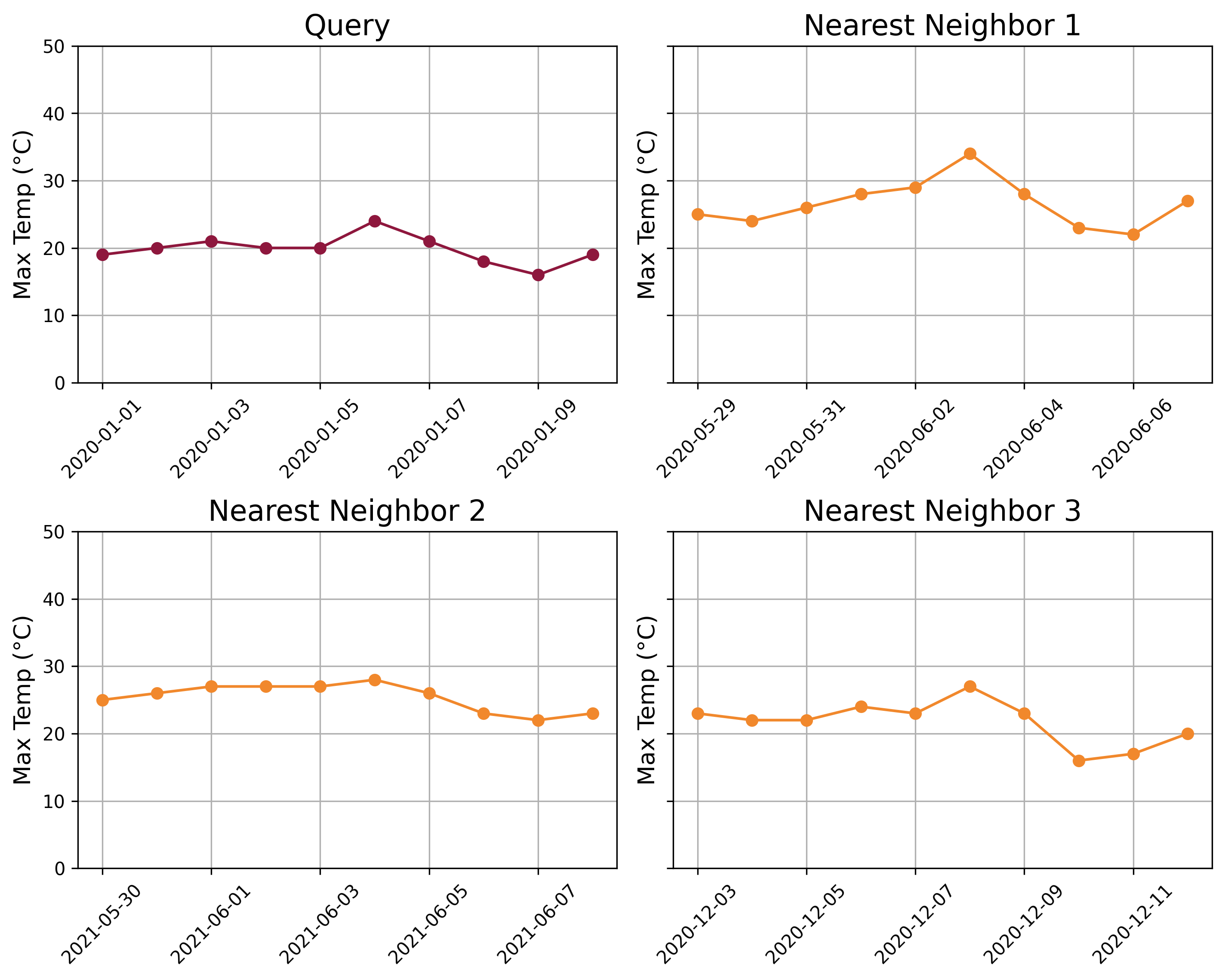
We can observe the similarities between the query and its nearest neighbors. The query time series shows a slight upward trend during the first 6 days, followed by a downward trend over the next 4 days. The three nearest neighbors exhibit similar patterns, effectively capturing the essence of the query subsequence.

It may seem surprising that the nearest neighbors to the query period from January 1st to January 10th, 2020, are not all from the same time of year (winter). In fact, two of the nearest neighbors fall in late May and early June. For example, while the average temperature during the query period is 19.8°C, the nearest neighbor on May 29, 2020, has an average temperature of 26.6°C.

This occurs because both the subsequences and the query are z-normalized before calculating the distance profile. Z-normalization removes magnitude differences, allowing the distance profile to focus on the shape of the temperature curve rather than the absolute values. This approach enables the identification of similar patterns in the data, regardless of differences in scale or offset.

MASS and STUMPY

Distance Profile involves calculating the distance between a query subsequence and all possible subsequences within a time series. While the basic concept can be implemented using NumPy, as shown above, this approach can become computationally expensive, especially for large datasets.

To address this, Mueen's Algorithm for Similarity Search (MASS) was developed as an optimized and highly efficient method for computing the distance profile. MASS leverages the Fast Fourier Transform (FFT) to significantly speed up the computation, making it well-suited for large-scale time series data. Essentially, MASS is a fast implementation of the Distance Profile algorithm, providing the same results but with much greater efficiency.

By using the stumpy package, which implements MASS, we can achieve scalable and rapid distance profile, enabling its use in real-world applications where performance and speed are critical.

Multi-Dimensional Distance Profile

The concept of distance profile can be extended to multivariate time series data, where each time point consists of multiple features or channels. This extension is crucial for performing similarity searches on multivariate time series, a common requirement in many real-world applications where data is collected across multiple channels simultaneously.

To compute a multi-dimensional distance profile, we can take one of two approaches:

1. Summing Individual Distance Profiles: Calculate the distance profile for each feature separately and then sum them to form a multi-dimensional distance profile.
   
2. Direct Multivariate Euclidean Distance: Compute the multivariate Euclidean distance directly across all features.
   

In our work, we opted for the first approach—summing the distance profiles of individual features. We acknowledge that this choice was somewhat arbitrary, and the impact of this decision on the results could be an interesting area for further exploration.

We utilized Mueen’s Algorithm for Similarity Search (MASS) to calculate the multi-dimensional matrix profile. Here’s how you can implement this approach:

def multi_dimensional_mass(
        query_subsequence: np.ndarray,
        time_series: np.ndarray
    ) -> np.ndarray:
    """
    Calculate the multi-dimensional matrix profile.

    Args:
        query_subsequence (np.ndarray): The query subsequence.
        time_series (np.ndarray): The time series.

    Returns:
        np.ndarray: The multi-dimensional matrix profile.
    """
    for dim in range(time_series.shape[1]):
        if dim == 0:
            profile = stumpy.core.mass(
                query_subsequence[:, dim], time_series[:, dim]
            )
        else:
            profile += stumpy.core.mass(
                query_subsequence[:, dim], time_series[:, dim]
            )
    return profile

Time-Step Classification

Time-step classification is a challenging task in time series analysis, where the goal is to assign a label to each individual time point within a sequence. This type of classification is crucial in various real-world applications, where the temporal dynamics of the data play a significant role in understanding and predicting outcomes.

The following are a couple of examples where time-step classification is applied:

1. Human Activity Recognition: In wearable technology and smart devices, time-step classification is used to identify and categorize human activities such as walking, running, or sitting, based on sensor data collected over time. Each time step in the sensor data corresponds to a specific activity label, enabling real-time monitoring and analysis.
   
2. ECG Signal Classification: In medical diagnostics, time-step classification is applied to ECG signals to detect and classify heartbeats as normal or indicative of various arrhythmias. Each time step in the ECG signal represents a moment in the cardiac cycle, and correctly labeling these steps is crucial for accurate diagnosis and treatment.
   

Problem Definition

Time-step classification involves assigning a label to each time step within a sequence, whether the data is univariate or multivariate. The dataset for this task typically includes the following characteristics:

• Input Features: The data consists of time series, which can be either univariate (single feature) or multivariate (multiple features).
• Label Assignment: For each time step, a specific label needs to be assigned, indicating the class or category of that particular time point.
• Training and Inference Data:
  • Training Data: Contains sequences that are fully labeled, providing the model with both the input features and the corresponding labels.
  • Test (Inference) Data: Contains sequences without labels, where the model needs to predict the label for each time step.
• Multiple Samples: The dataset may include multiple sequences, each representing different instances or subjects. For example, in Human Activity Recognition (HAR), each sequence might correspond to a different person performing various activities, with labels indicating the specific activity at each time step.
• Variable Sequence Lengths: The length of sequences can vary across both training and test data, meaning that each sample may have a different number of time steps.

Our goal is to train a model on the labeled training data so that it learns to accurately assign labels to each time step in the test data.

Distance Profile for Time-Step Classification

In this section, we explore how the Distance Profile technique, particularly through Mueen’s Algorithm for Similarity Search (MASS), can be adapted and applied to the task of time-step classification. By calculating the distance profile for each time step, we can effectively classify individual time points within a time series, enabling more precise and informed analysis across various domains.

The general approach is as follows:

1. Subsequence Querying: For each sequence in the test dataset, we break it down into smaller subsequences, or "queries." Each query represents a window of time steps within the sequence that we want to classify.
   
2. Finding Nearest Neighbors: For each query, we calculate its distance profile against the training dataset, identifying its k-nearest neighbors—subsequences in the training data that most closely match the query in terms of shape and pattern.
   
3. Label Assignment: The labels of these k-nearest neighbors are then used to assign a label to each time step in the query. This allows us to classify each time point in the test sequence based on the most similar patterns observed in the labeled training data.
   

Implementation Details

To adapt the MASS algorithm for Time-Step Classification, we made several key modifications to effectively handle the nuances of this task. These modifications ensure that the algorithm can accurately classify each time step in the test data by leveraging the labeled training data. Below are the critical components of our implementation:

Windows
Each sequence (i.e. sample) in the test data is divided into smaller windows to create the subsequences (queries) that will be classified. The window length is a tunable parameter, determined as a function of the minimum sequence length in the training data. This approach allows us to capture relevant patterns while maintaining consistency across varying sequence lengths.

Strides
To ensure comprehensive coverage of the test data, we allow overlapping windows to be created. The degree of overlap is controlled by a stride factor, enabling us to balance between computational efficiency and the thoroughness of the classification.

Distance Profile Calculation
For each window in the test data, we compute the distance profile over all subsequences from all samples in the training data. This is done using the MASS algorithm, which calculates the Euclidean distance on z-normalized data for each feature. The final distance measure for each subsequence is obtained by summing the distances across all features, ensuring that all aspects of the multivariate time series are considered.

k-Nearest Neighbors
Once the distance profile is calculated for each window in the test data, we identify the k-nearest neighbors from the training data based on the computed distances. These neighbors represent the most similar windows in the training set. The labels associated with these neighbors, which are one-hot encoded, are extracted for further processing.

Averaging Labels
A single time step in the test data may appear in multiple query windows, and for each window, we have k-nearest neighbors subsequences from the training data. To determine the final label for each time step index i within a query, we average the labels from corresponding index i across all the neighbor subsequences. This approach produces a set of label probabilities, from which the most likely label is assigned to the time step.

Limitations of the Approach

While the Distance Profile method for Time-Step Classification offers simplicity and interpretability, it has several limitations:

• Computational Expense: For large datasets, calculating distance profiles can be computationally intensive, potentially limiting scalability.
• Local Pattern Focus: Predictions depend entirely on the k-nearest neighbors identified. If these neighbors contain noisy/anomalous data (in features or labels), it can lead to noisy predictions.
• Parameter Sensitivity: Results can be sensitive to the choice of distance metric and the number of nearest neighbors (), requiring careful tuning.
• Computational Burden During Inference: Unlike models that learn during a training phase, this method performs all its computations during the inference phase. This can lead to slower predictions on large datasets compared to other complex models which, though potentially slow to train, are typically quick to make predictions once trained.

These limitations should be considered when applying this approach, particularly for large-scale or complex time series classification tasks.

Experiments

We tested the distance profile algorithm for time-step classification on five benchmarking datasets: EEG Eye State, HAR70+, HMM Continuous (synthetic), Occupancy Detection, and PAMAP2. These datasets, along with additional information about them, are available in the GitHub repository, which is also linked in the Datasets section of this publication.

Evaluation Results

The performance of the distance profile model was evaluated using a variety of metrics, including accuracy, weighted and macro precision, weighted and macro recall, weighted and macro F1-score, and weighted AUC. The results for each dataset are summarized in the table below:

As is common in benchmarking studies, we observe varying performance across different datasets. This variation likely reflects the inherent predictability of each dataset rather than specific strengths or weaknesses of the Distance Profile method. All models, including more complex ones, typically face similar patterns of relative difficulty across datasets.

Next, we compare the results of the Distance Profile model with those of LightGBM, a top-performing model in a comparative analysis conducted by this publication.

Comparison with LightGBM

For comparison, we now present the results from one of the top-performing model, LightGBM, from a comparative analysis conducted in this publication.

Note: Detailed results for all models in the Time Step Classification benchmark are available in this GitHub repository.

The LightGBM model also shows performance variability across datasets, with a notable correlation to the Distance Profile method's results. For instance, both models achieve their highest performance on the Occupancy Detection dataset.

Overall, LightGBM outperforms the Distance Profile method. The average of Macro Average F1-score for the Distance Profile model is 0.614, compared to 0.729 for LightGBM. This performance gap can be attributed to LightGBM's greater complexity and expressiveness, allowing it to capture more intricate data patterns than the simpler Distance Profile method.

Despite not matching LightGBM's accuracy, the Distance Profile model remains valuable for establishing benchmarks and quick prototyping. We recommend using it as a reference point during the development of more sophisticated models.

Summary

Distance Profile is a simple and versatile tool in time series data mining. It works by calculating the distance between a query subsequence and all other subsequences within a time series, forming the foundation for advanced analytical tasks.

We utilized Mueen's Algorithm for Similarity Search (MASS) for its efficiency and scalability, making it ideal for large real-world datasets. The process involves:

• Z-normalizing the time series and query to manage scale variations.
• Computing the Euclidean distance for each subsequence against the query.
• Supporting both univariate and multivariate data for comprehensive analysis.

While Distance Profile may not always achieve the highest accuracy compared to more complex models, it is invaluable for establishing strong baselines. Its simplicity and adaptability make it a must-have tool before advancing to more sophisticated methods.

Beyond time-step classification, Distance Profile is also effective for anomaly detection, motif discovery, and time series segmentation. Its broad applicability makes it an essential component of any data scientist's toolbox.

References

1. Law, Sean M. "STUMPY: A powerful and scalable Python library for time series data mining." Journal of Open Source Software 4, no. 39 (2019): 1504. Available at: https://stumpy.readthedocs.io.
2. Zhong, Sheng, and Abdullah Mueen. "MASS: distance profile of a query over a time series." Data Mining and Knowledge Discovery (2024): 1-27.