Introduction

Forecasting accurate electricity consumption is quite essential for handling mass energy management, maintaining stability of grids and optimize cost for millions of users, both at individual level and for the distribution agencies. Traditional time-series forecasting methods, such as statistical models or autoregressive models, often struggle to capture the complex, nonlinear and long-term dependencies in energy consumption data.

In this project, I use a Long Short-Term Memory Neural Network, to model and predict electricity consumption trends in Finland. The developed model process historical electricity consumption data, applies data normalization, learns intricate consumption patterns and makes future consumption predictions. A Flask-based web application is created which allows users to input no of past days to consider which would be used for training the model and generate future forecasts for specific number of days and visualize trends through graphical representations. Additionally, statistical insights, such as mean consumption, variability and trend direction, provide users with valuable decision-making tools.

Dataset Used

The dataset contains time-series data on electricity consumption in Finland which was recorded on an hourly basis. It includes timestamps in both UTC and UTC+03:00 time zones and covers a long period with over 52,000 rows. The key metric is electricity consumption, which fluctuates over time based on various factors such as demand patterns and seasonal changes. This data was used in analyzing energy consumption trends and future forecasting demands.

Tools and Frameworks needed

1. Programming Language

• Python: The language used for machine learning and deep learning.

2. Machine Learning & Deep Learning Frameworks

• TensorFlow/Keras: Used to build and train the Long Short-Term Memory model, enabling efficient handling of time-series data and sequential dependencies.

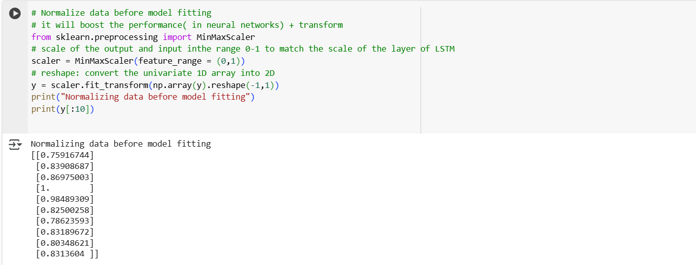
• Scikit-learn: Utilized for data preprocessing, normalization (MinMaxScaler), and statistical analysis to improve the quality of model inputs.

3. Data Processing & Visualization

• Pandas: Used for data manipulation and aggregation, ensuring the dataset is structured appropriately for training.

• NumPy: Provides efficient numerical computations for handling time-series sequences and transformations.

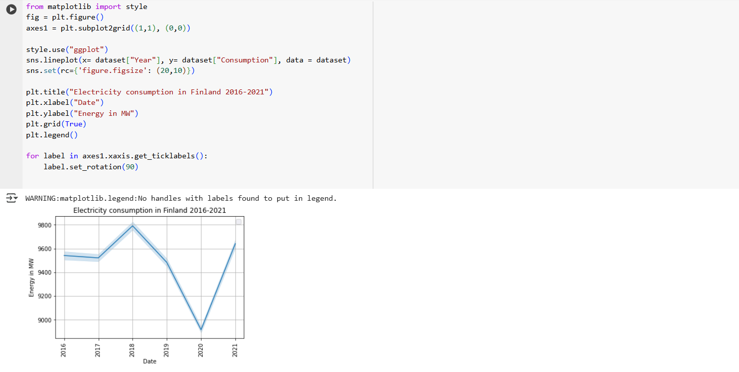
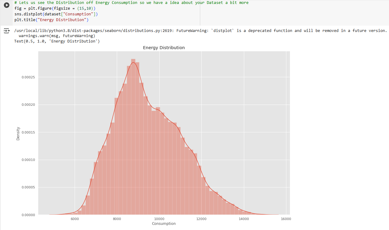
• Matplotlib & Seaborn: Used for visualizing past and predicted electricity consumption trends, helping to analyze forecasting performance.

4. Web Development & Deployment

• Flask: A lightweight Python web framework used to develop the user-friendly web application for model interaction and visualization.

• HTML and CSS: Used for the front-end interface, allowing users to input parameters and visualize forecasted results.

System Architecture

The electricity consumption forecasting system consists of a modular architecture, ensuring efficient data handling, accurate predictions and an intuitive user interface. It consists of three primary modules: Data Preprocessing, LSTM-based model training and Web-based deployment. Each module plays a pivotal role in utilizing existing electricity consumption data into developing a system which can be used for future forecast trends and actionable insights for energy planners.

1. Data Preprocessing Module

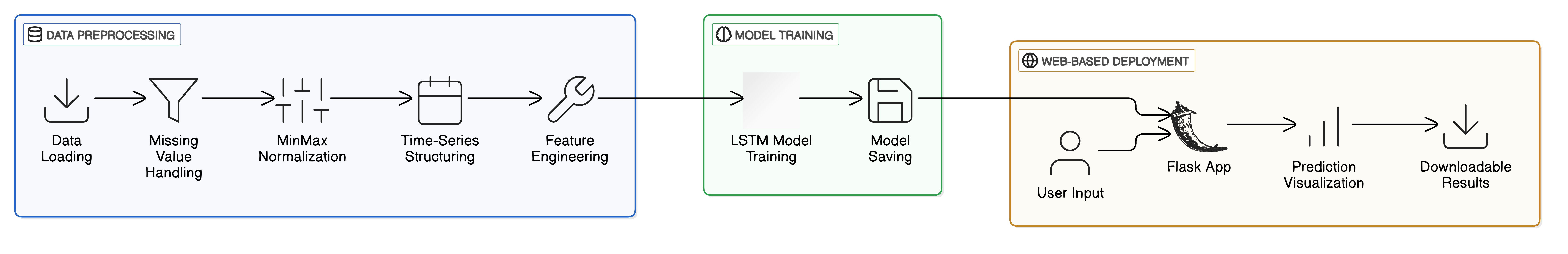
The data preprocessing module is responsible for handling raw historical electricity consumption data and preparing it for machine learning. The key tasks performed in this module include:

1.1 Loading and Cleaning Data

The system imports necessary libraries such as pandas, NumPy, Matplotlib, Seaborn, scikit-learn, Keras, and TensorFlow, then loads the electricity consumption dataset (events.csv) into a pandas DataFrame.

1.2 Exploratory Data Analysis (EDA)

• Displays first and last five rows (df.head(), df.tail()), checks data types and missing values (df.info()), and summarizes descriptive statistics (df.describe()).

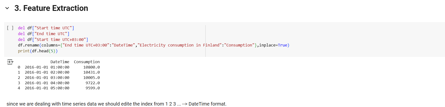
• Drops irrelevant columns ("Start time UTC", "End time UTC", "Start time UTC+03:00"), renaming the relevant time column as "DateTime" and consumption column as "Consumption".

• Extracts additional time-based features such as Month, Year, Date, Time, Week, and Day to aid in seasonal pattern detection.

• Sets "DateTime" as the DataFrame index and converts it into datetime objects for proper time-series structuring.

1.3 Data Visualization

• Time-Series Plots: Uses Seaborn’s lineplot to visualize electricity consumption over time.
  Also, generates individual plots for each year (2016-2021) to observe seasonal patterns.

• Distribution and Box Plots: Examines electricity consumption distributions and its variations across months, hours and years to identify trends and outliers.

1.4 Data Preparation for LSTM

• Downsampling: Aggregates hourly data into daily averages using resample("D").mean() to simplify forecasting.

• Normalization: Applies MinMaxScaler from scikit-learn to scale electricity consumption values between [0,1], improving LSTM model performance.

• Data Splitting: Divides the dataset into training, validation and testing to ensure model generalization.

2. LSTM-Based Model Training

The core of the forecasting system is a Long Short-Term Memory (LSTM) neural network, a type of recurrent neural network (RNN) designed specifically for time-series forecasting. The training process involves several key steps:

2.1 Dataset Preparation for Model Training

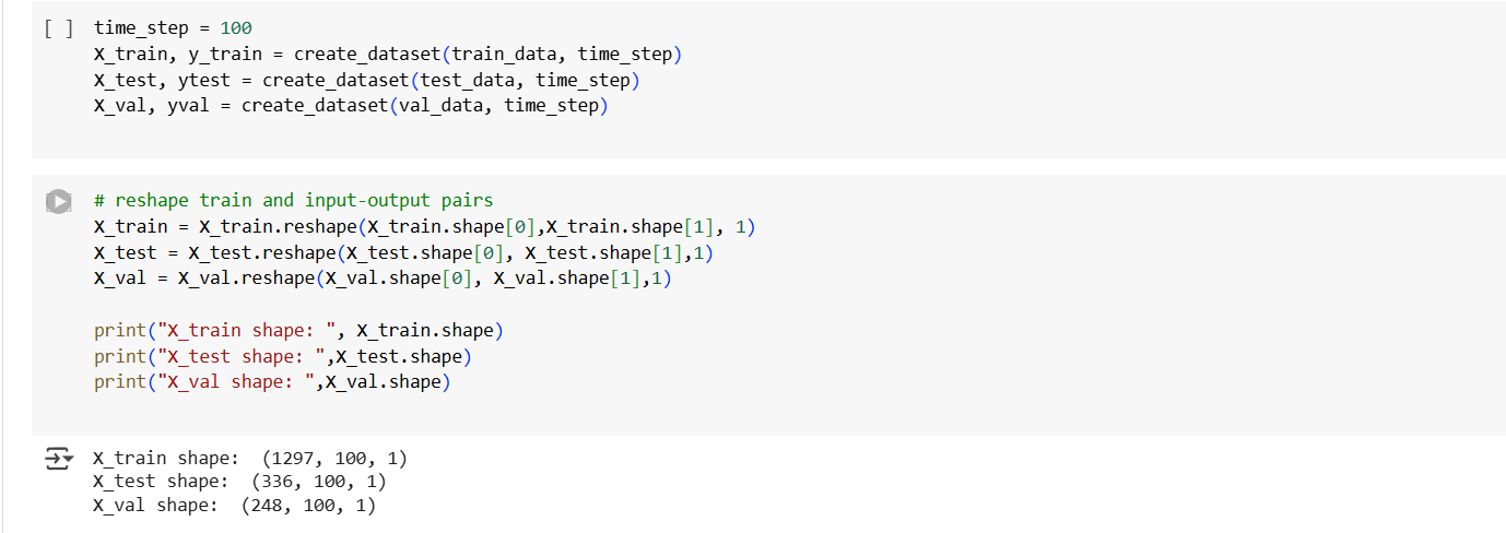
The preprocessed and normalized time-series data is structured into sequences where a set number of past observations are used to predict future values.

2.2 Model Architecture

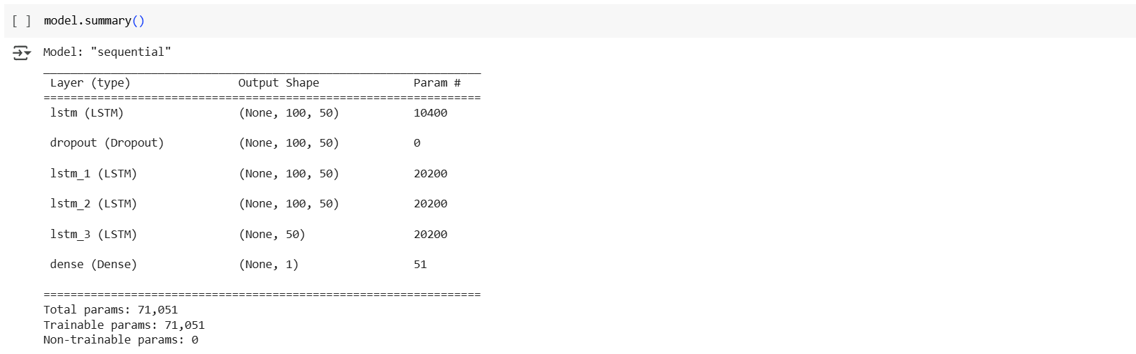
The LSTM model is implemented using Keras Sequential API, consisting of:

• Four LSTM layers to capture temporal dependencies.

• Dropout regularization layers to reduce overfitting.

• Dense output layer with a single neuron for forecasting one-step-ahead consumption.

2.3 Model Compilation and Training

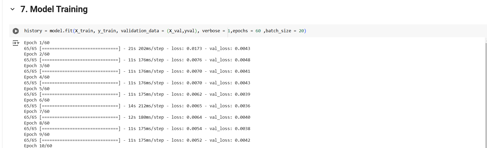
• The model is compiled using the Adam optimizer and Mean Squared Error (MSE) loss function.

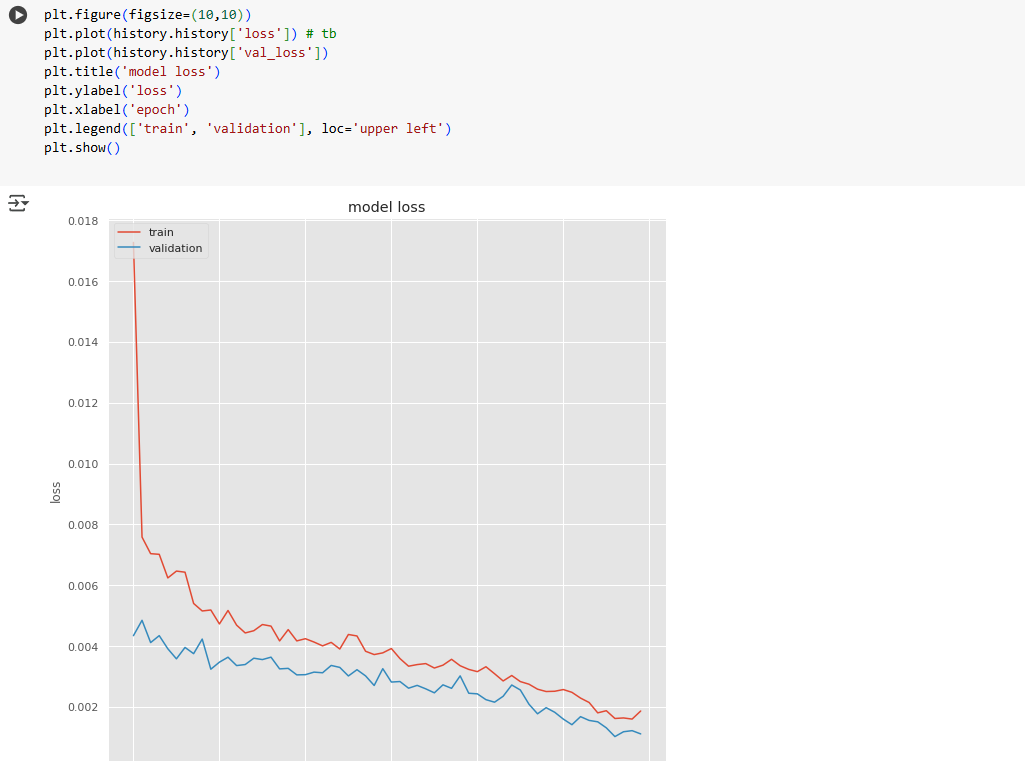
• The training process is monitored over multiple epochs, with model performance evaluated on the validation set.

2.4 Model Evaluation and Performance Metrics

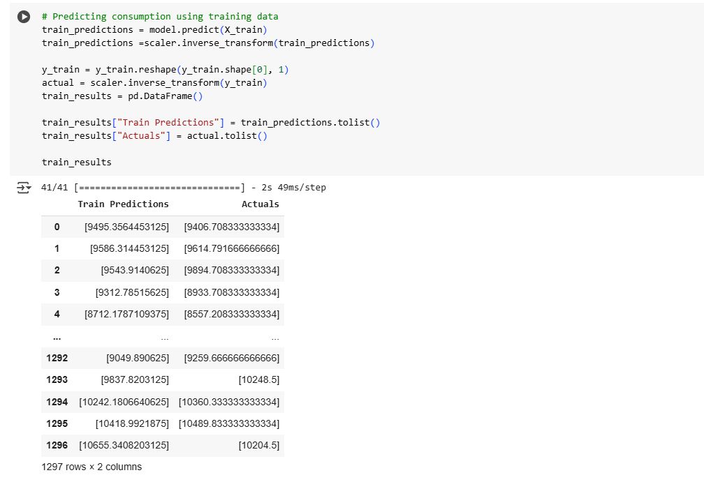
• The trained model is tested on unseen validation data, with predictions being inverse-transformed to the original scale.

• The model’s accuracy is measured using Mean Squared Error for training and validation datasets.

3. Web-Based Deployment using Flask

To make the forecasting system accessible and interactive, a Flask-based web application serves as the front-end interface, allowing users to interact with the model seamlessly. The web application facilitates:

3.1 User Input Handling

• Users can specify forecasting parameters, such as the number of future days to predict.

3.2 Historical Data Retrieval & Prediction Generation

• The system retrieves relevant past electricity consumption data.

• The trained LSTM model processes input data and generates forecasts for the specified future period.

3.3 Visualization & Result Presentation

• The system provides comprehensive visual representations of actual vs. predicted consumption trends.

Key plots include:

• Predicted vs. Actual Consumption: Separate plots for training, validation, and testing datasets.

• Combined Time-Series Forecast: Displays both historical and predicted values for a comprehensive trend analysis.

• Key statistical insights, including mean, variance, seasonal trends, and direction of change, are provided.

Implementation

This section describes the implementation of our electricity consumption forecasting system, based on the app.py file.

1. Data Preprocessing

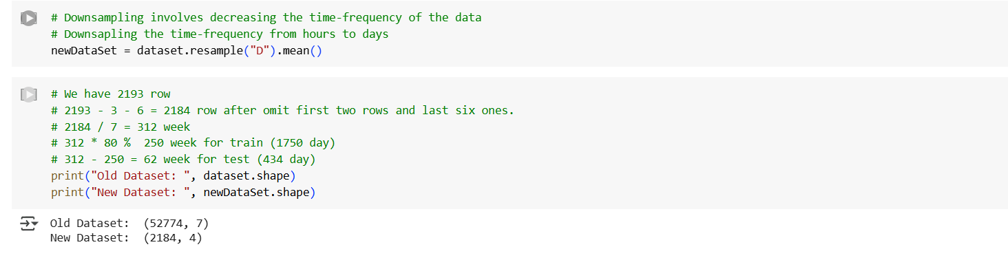
The dataset is loaded from data/events.csv, where relevant columns are renamed and timestamps are converted to datetime format. The data is aggregated at the daily level using resampling and normalization is applied using MinMaxScaler to improve model efficiency.

2. Forecasting Process

A pre-trained LSTM model stored in model/lstm_model.h5 is used for predictions. The forecasting function follows these steps:

1. Extracts a sequence of past consumption values based on user input.

2. Feeds the sequence into the model to generate forecasts.

3. Iteratively predicts the specified number of future days.

4. Inversely transforms the predicted values back to their original scale.

3. Web Application

The Flask application provides an interface for users to input forecasting parameters. The process includes:

• Users specify the number of past and future days.

• The system processes the input and retrieves corresponding data.

• The model generates forecasts and statistical metrics such as mean, standard deviation, and trend direction.

• A visualization of the forecast is generated using Matplotlib and displayed as a base64-encoded image in the results page.

4. Results Presentation

The results are displayed on the results.html page, which includes:

• A tabular representation of predicted values.

• Statistical insights including mean, range, and trend assessment.

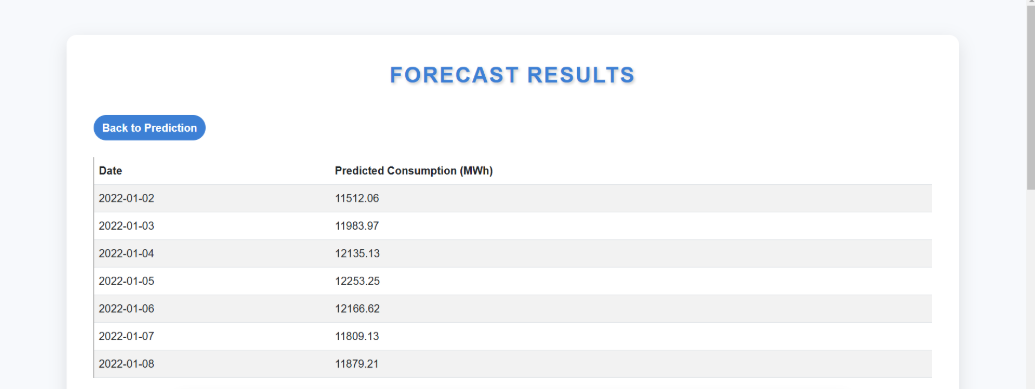
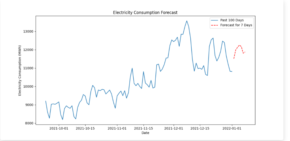
• A graphical comparison of past and forecasted consumption trends.

• Users can download the results for further analysis.

5. Deployment

The application is executed as a Flask server with debugging enabled for development. It runs on http://127.0.0.1:5000/, allowing external access if necessary. It is containerized using Docker for seamless deployment across different environments.

Results

The results indicate that the model is able to effectively capture long-term dependencies and fluctuations in electricity demand. By leveraging sequential learning, the model demonstrates improved accuracy over traditional statistical forecasting methods. The predictions generated by the model closely follow the actual consumption patterns, with minimal deviations observed in short-term forecasts.

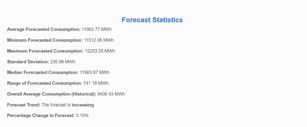
To further assess the model’s performance, statistical insights were extracted from the forecasted results. These include:

• Mean Forecasted Consumption: The average electricity demand predicted by the model.

• Minimum and Maximum Consumption Values: Identifying the range of fluctuations in the forecasted period.

• Standard Deviation and Variability: Analyzing how stable or volatile electricity consumption is over time.

• Trend Direction: Indicating whether electricity consumption is expected to increase or decrease in the coming days.

• Percentage Change in Forecasted Values: Providing insights into the expected shift in energy demand over time.

Conclusion

The model was well able to capture trends but despite its effectiveness, the model possess certain limitations. External factors such as temperature fluctuations, economic trends and adherence to policy changes were not included in the dataset, which may impact the accuracy of long-term forecasts, significantly. Additionally, LSTMs, while powerful, can be computationally expensive and struggle with very long-term predictions due to accumulated errors over time. Another limitation is the reliance on single-variable forecasting, as the model currently predicts electricity consumption using only past values of the same variable.

Github Repository :- VoltVision