Stock Price Forecasting With Exogenous Variables

Introduction & Motivation

Stock market prediction, the act of determining the future value of a company stock or any other financial instrument traded on an exchange, has always been a subject of interest within stakeholders. Today, we perform this task using machine learning.

However, time series forecasting is not always a straightforward task, and many data scientists struggle to obtain meaningful results. This publication displays a step-by-step approach, including exogenous variables, to increase each model's forecasting accuracy. By incorporating additional relevant factors beyond historical prices, we aim to enhance the precision and reliability of predictions. Through this exploration, we provide valuable insights and methodologies that can serve as a foundation for future advancements in stock market prediction using machine learning.

1. Data Collection & Preprocessing

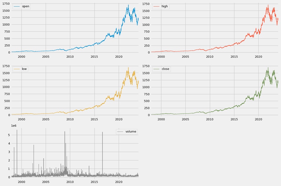
The first step was to collect daily stock price data. The data was downloaded for free from Yahoo! Finance using an API. The dataset includes several decades of data available for most exchanges. It contains six basic price attributes: open, high, low, close, adjusted close, and volume (in USD), as well as an index date column in the YYYY-MM-DD format. In this project, we focused on forecasting the closing prices. The company of choice was Mettler-Toledo International Inc., listed on the New York Stock Exchange (ticker symbol: MTD).

Since there were no dividends, the close and adjusted close prices were identical, so the latter were dropped.

Not all dates were included in the dataframe. These missing records were not trading days (weekends, holidays, etc.). Linear interpolation was implemented to add these rows and fill missing values.

2. Outlier Detection

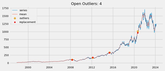
Outliers were detected for each variable except volume. A Z-score test was applied to identify these observations, which were then modified to be the mean of the preceding 50 values (rolling window size). As is common practice, a Z-score threshold greater than 3 was used to define outliers. Below is an example using open prices.

3. Feature Engineering

To enrich the dataset and capture more information and patterns, feature augmentation was performed by adding new exogenous features. This step aimed to improve both model training and prediction accuracy. For stock prices, techniques such as differencing, trend indicators, rolling statistics, and transformations (e.g., percentile, Z-score, logarithm) can be applied. Implementing technical indicators is also a common form of feature engineering. Some of the features used included:

• market capitalization;
• stochastic oscillator;
• cumulative change;
• exponential moving averages;
• simple moving averages;
• William's %R (William's percent range),
• end of month indicator;
• daily variation;
• weekday, quarter, year, etc.

After that, some basic EDA (exploratory data analysis) was performed to visualize our new features and search for any patterns throughout the historical data.

4. Feature Selection

A crucial step in our analysis was selecting the most relevant and informative features for the forecasting models while discarding those that were redundant or uninformative. This process offers several advantages: it reduces model complexity, enhances learning efficiency, and can even improve predictive performance by minimizing noise.

All introduced features, as well as the target variable, were continuous. We applied correlation analysis, p-values, and the mutual information method. By combining these scores, we were able to identify the most relevant variables. Below are the selected features based on the top scores ( = 15).

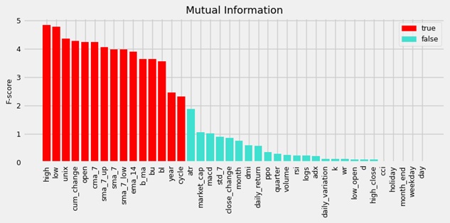
The following chart displays the selected features based on the top 40th percentile of scores. Both selection approaches produced very similar results, with the percentile method returning one additional feature.

The supported features had very high F-scores, meaning they shared an arbitrarily large amount of data, and the dependence between random variables was significant. The technical indicators with white noise signals tended to have almost no correlation. They had means equal to zero and were identically distributed. This type of feature had the same variance and no visible trends in line plots. The datetime features, such as day of the week, holiday, and day of the month, also had the lowest scores. In general, features with a false mask tended to have low correlation coefficients with the target price, which is what we would expect. All variables with a p-value greater than 0.05 (or 5%) showed false support.

The selected features were exported as a new dataset to a CSV file. More details to this stage can be found in this Jupyter notebook.

5. SARIMAX Estimator

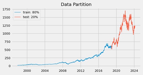
The first model introduced for stock price prediction was the SARIMAX algorithm. This model does not require data scaling or normalization. The endogenous variable (i.e., the one to be predicted) was the closing stock price, while the remaining features served as exogenous variables. For each approach, the data was split using an 80/20 ratio.

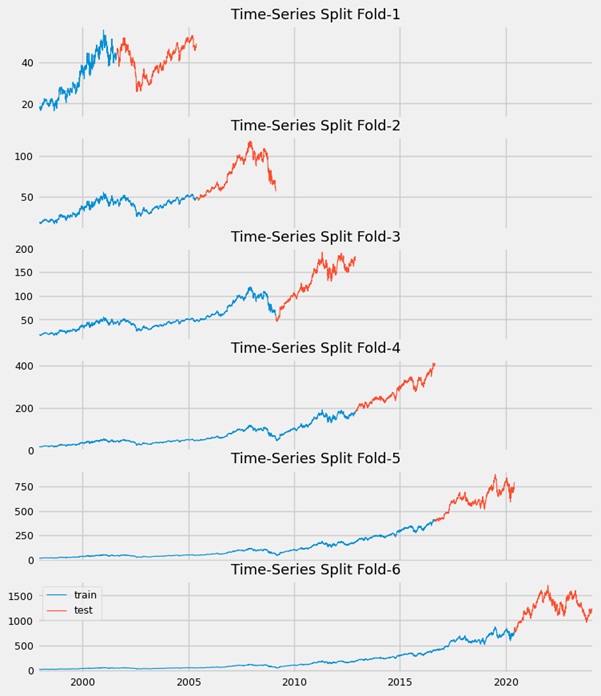
To find the optimal model configuration (i.e., the orders), a stepwise fitting approach was applied using auto-ARIMA. No specific trend was detected in the time series. The model’s performance was evaluated using several metrics: RMSE, 6-fold cross-validation, R², MAE, MAPE. The chart below illustrates the train/test split used for cross-validation score evaluation within our time series.

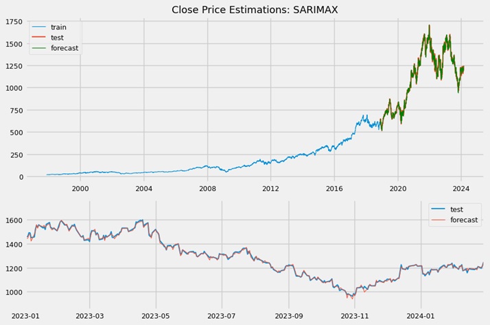
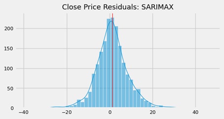
This regressor performed very well and appeared promising. The predicted values closely overlapped the actual values, with the prediction line nearly matching the true line. The price residuals followed a near-perfect normal distribution, with only a slight positive skew. The mean value of residuals were very close to zero (more details in Jupyter notebook).

6. RNN & LSTM Estimators

The next models used were artificial neural networks developed in TensorFlow, specifically RNN and LSTM regressors, both of which required appropriate transformations. The dataset was reframed into a supervised form, meaning that lag observations needed to be generated by shifting the target variable. Copies of columns were created and either pushed forward (with NaN rows added to the front) or pulled back (with NaN rows added to the back). The augmented dataset was shorter by the number of lags (). This time, the dataset variables were scaled to the [0, 1] range; note that the predictions need to be inverted back to the original range. Both architectures are introduced in this notebook. Here are the results for the RNN model:

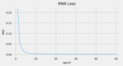
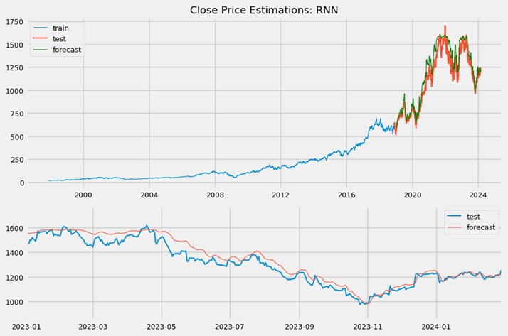
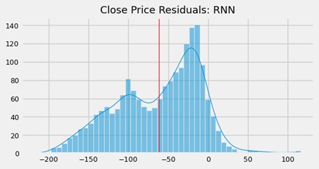
This predictor proved to be ineffective, as the estimated price line did not overlap with the true line. The residuals exhibited a highly uneven, trimodal distribution with significant positive skewness. In contrast, the LSTM model was more sophisticated, both in terms of its architecture and the flow of information through the unit. Here are the results obtained for the model:

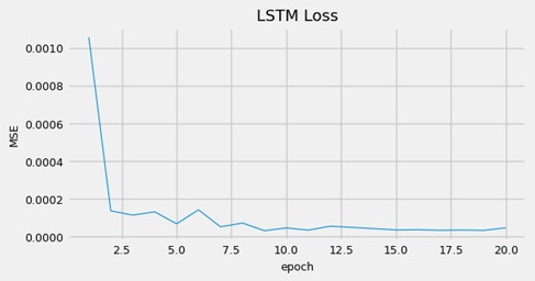
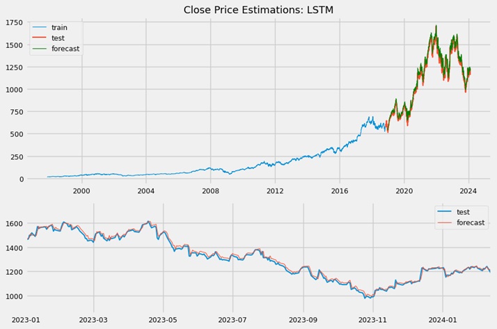
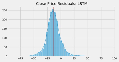
This network performed much better than the previous RNN model and was more reasonable in its predictions. The residuals were more evenly distributed, with a slight negative skewness. Positive residuals were larger because the forecasted line was shifted higher than the true line. The network’s memory cells were better at capturing and processing sequential information compared to the RNN. Introducing a different number of lags could potentially improve the model’s performance.

7. Prophet Estimator

Another time series estimator implemented was Facebook's Prophet model. Similar to SARIMAX, it does not require data scaling or normalization. Unlike ARIMA, this algorithm can capture trend changes. By nature, it is univariate and takes into account different seasonalities and holidays. It can also function as an outlier detector. By setting most seasonality components to 'auto', leaving holidays unspecified, and using a multiplicative seasonality mode, the predictions were as follows (the green area represents the confidence intervals).

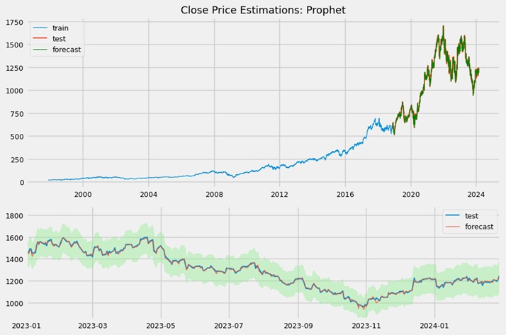
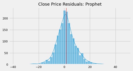
The forecasted trend line fit well to the data. The residuals were well balanced, exhibiting a symmetrical shape and a Gaussian distribution. Overall, the Prophet model performed accurately and showed promising results for our data. More details about the model developing are available in this Jupyter notebook.

8. Scikit-learn Estimators

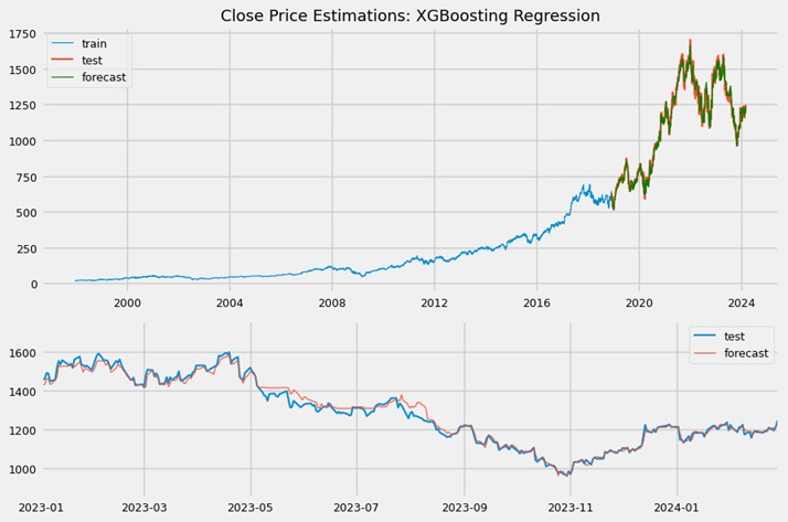
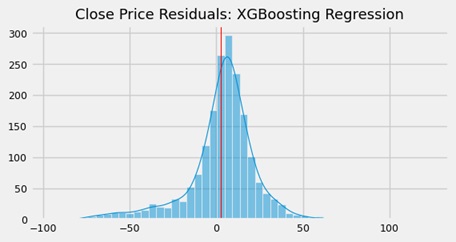
Last notebook displays estimations using different scikit-learn models.

8a. Linear Estimator

Linear regression does not require data preprocessing or normalizing.

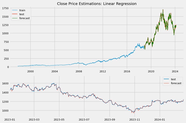
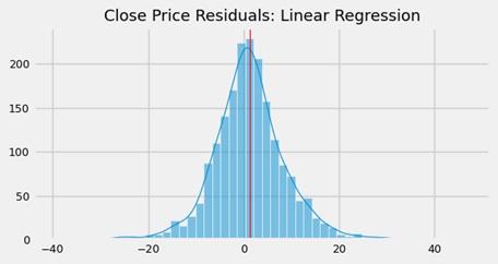
Despite its simplicity, this model had surprisingly great performance. The results confirm our belief that the dataset's variables were linearly correlated and heavily related to the response. The feature selection was determined correctly and there was no need to include penalty or regularization terms. The histogram displayed residuals with almost Gaussian distribution.

8b. Data Preprocessing & Splitting

Most machine learning models for time series forecasting still require reframing the dataset into a supervised form (similar to the format used for the previous neural networks). To determine the optimal number of lags, the Augmented Dickey-Fuller (ADF) test was applied. The information criteria method (AIC) was used to select the lag length that minimizes the corresponding information criterion. A dataset that is too large can introduce noise and make the model overly complex, while a dataset that is too small might lack sufficient historical information for accurate predictions. The 80/20 split ratio was maintained. Additionally, the next models required scaling the data to the [0, 1] range.

8c. Support Vector Estimator

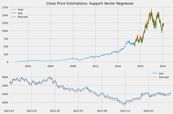
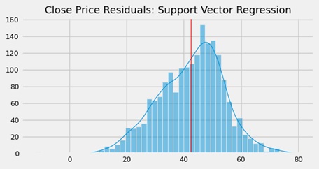
Even after hyperparameter tuning, the support vector estimator did not perform well. While the predicted trend line closely resembled the true one, it was negatively shifted. The residuals showed an uneven distribution, with all values being positive due to this shift.

8d. XGBoosting Estimator

The last model's predicted trend line had a good fit. The residuals were much more balanced compared to the support vector model. Still, the linear regression out-performed this estimator and returned much lesser price deviations.

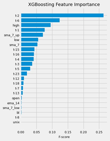
We can spot on this bar plot that the lag variables (shifted target ) generated in the supervised dataframe were the most numerous and how crucial they were for different machine learning algorithms. They contained useful information about the target's patterns.

The following table displays evaluation metrics for each implemented model.

9. Conclusions

This work addressed a time series prediction problem for stock prices. To tackle the task, seven diverse and commonly used machine learning models were introduced. Their performance was evaluated using basic regression metrics and plots.

Among all the estimation models demonstrated, the RNN and support vector models proved to be the least effective. Surprisingly, the linear regression model, due to its simplicity, achieved great accuracy, which indicated that the key assumptions were met. The EDA process showed that the engineered, independent features significantly enriched the dataset with useful information and were linearly correlated with the dependent variable (closing price). Linear regression is also sensitive to influential points (outliers) which were removed correctly. The feature selection process, performed in the final phase of the EDA notebook, was carried out effectively, and the selected variables did not introduce unnecessary noise into the dataset.

Although the SARIMAX regressor had practically the same performance and is much more widely applied among the data science community, the final choice should be for linear regression. This model is much more simple to develop, easy to understand, requires much less data preprocessing and computational power. The cross-validation scores indicate the linear regressoin works better to unseen data compared to the SARIMAX.

The project was a success, with the time series predictions achieving high accuracy. Additional conclusions include:

• Adding extra variables (engineering features) proved to be highly beneficial. This enriched the dataset, provided more information, and therefore improved regression performance.
• Feature selecting was crucial. This process allowed us to eliminate unnecessary variables which could possibly cause biased or unstable estimates of regression coefficients. Most time-related predictors (quarter, month, holidays, etc.) turned out to be the least useful. Features with little to no variance also failed to provide meaningful information. A combination of tests helped confirm our choices.
• The characteristics of stock prices were linear. This was demonstrated through feature selection and the linear estimator, which assumes linear relationship and homoscedasticity.

References

1. Adil Moghar, Mhamed Hamiche, 2020, Stock Market Using LSTM Recurrent Neural Network, Full Text
2. Ruobing Zhang, 2022, LSTM-based Stock Prediction Modeling and Analysis, Full Text
3. https://finance.yahoo.com/quote/MTD/
4. https://neptune.ai/blog/arima-vs-prophet-vs-lstm

Code & Resources

All Jupyter notebooks and code are available in this GitHub repo