# Abstract This paper presents a novel approach to measuring fashion item similarity using a Siamese neural network trained on the Fashion MNIST dataset. By leveraging a custom contrastive loss function, the proposed model learns to discern fine-grained visual similarities and differences between pairs of clothing images. In this framework, each branch of the Siamese network processes one of the two input images, and the final distance metric reflects how closely related the items appear. Our experimental results demonstrate that the network effectively captures subtle variations in clothing attributes, such as shape and texture. This similarity determination method has potential applications in product recommendation systems, automated cataloging, and user-driven visual search, thus contributing a robust technique for fashion-focused image analysis. Results showed a validation accuracy of 89,9%, alongside a test accuracy of 89,1%, indicating that even with a relatively simple feedforward design, the model reliably distinguishes between a broad range of clothing categories. These findings highlight the potential of compact neural architectures for recommendation systems, inventory organization, and personalized search, suggesting avenues for future work that could integrate more extensive or high-resolution fashion datasets. --DIVIDER--# Introduction In recent years, the booming online retail industry has prompted a growing demand for advanced tools to help consumers and businesses navigate vast fashion catalogs. One core challenge lies in accurately identifying and quantifying the visual similarity between apparel items. Whether assisting users in finding complementary outfits or enabling brands to organize and tag inventory, the capability to compare clothing items based on shared features—such as color, pattern, and silhouette—offers clear advantages for both consumers and retailers. This need has driven research into visual recognition methods that go beyond simple categorical classifications, focusing instead on measuring more nuanced degrees of similarity. 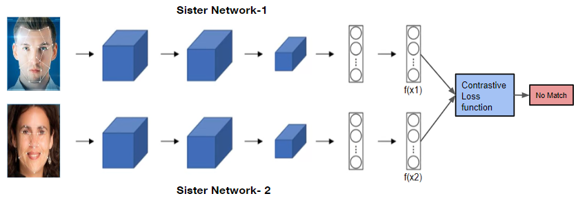Siamese neural networks have emerged as a powerful solution to address this challenge, particularly because they learn a metric space where similar inputs map close together and dissimilar inputs lie far apart. Unlike traditional classification models that assign discrete labels, Siamese networks process pairs of images in parallel with shared weights, enabling them to extract comparable high-level features from each input. This characteristic is especially valuable in domains like fashion, where the inherent variability of styles and subtle design differences demand a model capable of capturing fine-grained visual cues. ![](https://miro.medium.com/v2/resize:fit:1400/0*lgjFPlTjPjiW4ziu.png)

Figure 1. Siamese Network Architecture

Central to training a Siamese network for similarity tasks is the contrastive loss function. Rather than penalizing classification errors in the conventional sense, contrastive loss drives the distance between representations of similar pairs to be small and dissimilar pairs to be large. By enforcing this distance-based objective, the network efficiently learns to embed images into a feature space that reflects their semantic similarity. In the context of fashion, this means that two visually similar clothing items—despite differences in brand, texture, or minor design details—will be mapped closer together in the learned embedding space, while those with contrasting features will be placed farther apart. This paper explores the use of Siamese networks with contrastive loss for the task of fashion item similarity, demonstrating its effectiveness on a widely used benchmark dataset. The proposed approach offers a robust, scalable solution that can be integrated into recommendation systems, visual search engines, and automated product organization pipelines, facilitating more intelligent and user-friendly interactions within the fashion ecosystem. --DIVIDER--# Methodology ## 1. 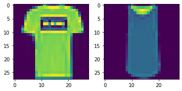Data Collection and Preprocessing This work employs the Fashion MNIST dataset, which consists of 60,000 training images and 10,000 test images in 10 classes of clothing items. Although larger or more specialized fashion datasets can capture greater visual complexity, employing Fashion MNIST provides an accessible and efficient platform for exploring similarity modeling. Notably, small datasets can still be sufficient for training when the model architecture and loss functions are carefully chosen, as observed in practice. Prior to training, each image is resized to a uniform dimension (28×28 pixels) and normalized, helping to stabilize learning by setting consistent input ranges. ![Fashion MNIST Dataset plot](download.png)

Figure 2. Fashion MNIST Dataset.

## 2. Base Network In this work, the base network is implemented as a Multilayer Perceptron (MLP), a type of feedforward neural network composed of fully connected layers that transform input data through successive nonlinear transformations. An MLP is particularly effective for a broad range of supervised learning tasks, such as image classification and similarity detection, due to its ability to capture complex relationships in the data. Specifically, the Fashion MNIST images are first flattened from their original 28×28 shape into 784-dimensional vectors. These vectors serve as the input to multiple Dense (i.e., fully connected) layers, each followed by an activation function (e.g., ReLU) to enable nonlinear learning. Dropout layers are introduced between the dense layers to reduce overfitting by randomly deactivating subsets of neurons during training. This approach is aligned with standard practices in neural network design, where fully connected layers can capture and combine abstract features while dropout provides essential regularization

Table 1. Summary of the Base Architecture used in the Proposed System.

| Layer Name | Type | Input Shape | Output Shape | Notes | |--------------------|------------|----------------|----------------|-----------------------------| | base_input | InputLayer | (None, 28, 28) | (None, 28, 28) | Initial input for 2D images | | flatten_input | Flatten | (None, 28, 28) | (None, 784) | Converts 2D to 1D vector | | first_base_dense | Dense | (None, 784) | (None, 128) | Fully connected layer | | first_dropout | Dropout | (None, 128) | (None, 128) | Prevents overfitting | | second_base_dense | Dense | (None, 128) | (None, 128) | Fully connected layer | | second_dropout | Dropout | (None, 128) | (None, 128) | Regularization step | | third_base_dense | Dense | (None, 128) | (None, 128) | Final embedding layer | ## 3. 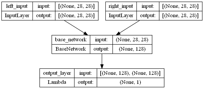Siamese Network A Siamese network comprises two identical sub-networks (i.e., two copies of the base CNN) that share weights, effectively acting as "twin" networks. During training, each sub-network receives one of the two images in a pair, passing the inputs through the same feature extraction pipeline. This shared-weights design ensures that the resulting embeddings are learned in a consistent feature space, making pairwise comparisons more reliable. The final output of each sub-network is a latent representation of the input image, and a distance metric—commonly Euclidean—measures how similar or dissimilar the two embedding vectors are. By focusing on determining whether two inputs belong to the same semantic category (or share high visual resemblance), Siamese networks naturally lend themselves to the task of fashion similarity.

Figure 3. Siamese Network Architecture used in the Proposed System.

## 4. Contrastive Loss Unlike classification tasks that rely on cross-entropy loss, Siamese networks benefit from a distance-based learning objective. The contrastive loss function compels the model to embed visually similar pairs closer together while pushing dissimilar pairs farther apart. Formally, for an image pair with label Y (0 for similar, 1 for dissimilar), and distance D between their embeddings, the contrastive loss is computed as: $$ L = (1 - Y) \times \frac{1}{2}\bigl(D^2\bigr) \;+\; Y \times \frac{1}{2}\Bigl(\max\bigl(0, m - D\bigr)^2\Bigr) $$ where: - **L**: The computed loss value, encouraging similar items to remain close and dissimilar items to remain sufficiently distant. - **Y**: A binary label indicating pair similarity. If $Y = 0$, the pair is similar and their distance $D$ should be minimized. If $Y = 1$, the pair is dissimilar and their distance $D$ should exceed the margin $m$. - **D**: The distance (e.g., Euclidean) between the latent representations of two items. - **m**: The margin that enforces a minimum separation between dissimilar item pairs. When $Y = 0$, the term $\tfrac{1}{2} D^2$ is minimized, penalizing large distances between visually or semantically similar examples. Conversely, when $Y = 1$, the term $\tfrac{1}{2}\bigl(\max(0, m - D)^2\bigr)$ is minimized, penalizing distances below the margin $m$. This formulation ensures that the network learns to produce embeddings that meaningfully reflect visual similarity or dissimilarity. Through this formulation, the model is penalized for assigning large distances to similar pairs or small distances to dissimilar pairs, thus learning a feature space that aligns with intuitive notions of similarity and difference. unifying these components—data preprocessing, a robust base MLP, weight-sharing Siamese architecture, and contrastive loss—the proposed methodology provides a scalable and efficient means of measuring fashion similarity. --DIVIDER--# Experiments ### Load the Dataset--DIVIDER-- In this section, we import the Fashion MNIST dataset and split off a portion of the test set to serve as a validation set. Each image is then converted to float32 and normalized by dividing by 255.0. This ensures that the network trains on standardized input values, helping it converge more stably. ```python from tensorflow.keras.datasets import fashion_mnist from sklearn.model_selection import train_test_split # load the dataset (train_images, train_labels), (test_images, test_labels) = fashion_mnist.load_data() # split to test and validation test_images, val_images, test_labels, val_labels = train_test_split(test_images, test_labels, test_size=.5, random_state=0) # prepare train and test sets train_images = train_images.astype('float32') val_images = val_images.astype('float32') test_images = test_images.astype('float32') # normalize values train_images = train_images / 255. val_images = val_images / 255. test_images = test_images / 255. ``` --DIVIDER--### Prepare the Dataset--DIVIDER-- Here, we define functions to pair up images: • ***create_pairs***: Builds positive (same class) and negative (different class) image pairs by randomly selecting images from the specified labels. • ***create_pairs_on_set***: Applies create_pairs to a given set (training/validation/test), returning pairs of images (shape: [?, 2, 28, 28]) and binary labels (1 for same, 0 for different). This pairing process is essential for training the Siamese network with contrastive loss. ```python import random import numpy as np def create_pairs(images, labels): """ Create a positive and negative pair images Parameter ---------- images: numpy array of images labels: numpy array of labels Return ---------- pair_images: numpy array of random paired image pair_labels: numpy array of binary value (1 is positive, 0 is negative) """ pair_images, pair_labels = [], [] n = min([len(labels[l]) for l in range(10)]) - 1 for l in range(10): for i in range(n): # create positive pair image z1, z2 = labels[l][i], labels[l][i + 1] pair_images += [[images[z1], images[z2]]] inc = random.randrange(1, 10) dn = (l + inc) % 10 # create negative pair image z1, z2 = labels[l][i], labels[dn][i] pair_images += [[images[z1], images[z2]]] pair_labels += [1,0] return np.array(pair_images), np.array(pair_labels) def create_pairs_on_set(images, labels): """ Create a set for training data Parameter ---------- images: numpy array of images labels: numpy array of labels Return ---------- pairs: numpy array of random paired image y: numpy array of binary value (1 is positive, 0 is negative) """ digit = [np.where(labels == i)[0] for i in range(10)] pairs, y = create_pairs(images, digit) y = y.astype('float32') return pairs, y ``` After that, we generate pairs for the training, validation, and test sets. We invoke ***create_pairs_on_set*** on train_images, val_images, and test_images. This produces arrays of image pairs along with a matching array of labels, used later in training. --DIVIDER--```python # create pairs on train, validation and test sets train_image_pairs, train_label_pairs = create_pairs_on_set(train_images, train_labels) val_image_pairs, val_label_pairs = create_pairs_on_set(val_images, val_labels) test_image_pairs, test_label_pairs = create_pairs_on_set(test_images, test_labels) ``` The ***show_image*** function displays a pair of images side by side. It’s a small utility for visualizing whether the pair is “the same” or “not the same” based on our labels. --DIVIDER--```python def show_image(anchor_image, image): """ Display pair data Parameter ---------- image: a set of image pair ax: an integer for axis Return ---------- None """ _, axs = plt.subplots(1,2) axs[0].imshow(anchor_image) axs[0].grid(False) axs[1].imshow(image) axs[1].grid(False) plt.show() ``` Next, we pick an index (here, zero) to see an example pair and print whether the pair is in the same class. --DIVIDER--```python # array index index = 0 # show images at this index show_image(train_image_pairs[index][0], train_image_pairs[index][1]) print('The train pair is', 'the same' if train_label_pairs[index] == 1 else 'not the same') # The train pair is the same ``` ![pair.png](pair.png)

Figure 4. Train Dataset Example at Index 0.

--DIVIDER--### Develop Base Network--DIVIDER-- We define a BaseNetwork class, which inherits from keras.Model. Inside, we flatten the input images and pass them through a combination of Dense and Dropout layers. This MLP architecture transforms each 2D fashion image into a 128-dimensional embedding. After we instantiate the BaseNetwork, we build a model (base_model) around it—primarily for visualization—and generate a plot of the layer structure. ```python from tensorflow import keras from keras import Model from keras import layers from keras.utils.vis_utils import plot_model class BaseNetwork(Model): def __init__(self): super(BaseNetwork, self).__init__() self.flatten = layers.Flatten(name='flatten') self.d1 = layers.Dropout(.2, name='dropout_1') self.fc1 = layers.Dense(256, activation='relu', name='fully_1') self.d2 = layers.Dropout(.2, name='dropout_2') self.fc2 = layers.Dense(128, activation='relu', name='fully_2') def call(self, inputs): x = self.flatten(inputs) x = self.d1(x) x = self.fc1(x) x = self.d2(x) return self.fc2(x) base_network = BaseNetwork() ``` We set up an Input layer matching the image shape (28×28) and pass it through our BaseNetwork. The plot_model call creates a visual diagram of this architecture. --DIVIDER--```python input_shape = train_images[0].shape inputs = layers.Input(shape=input_shape) # create base model and display model layer output = base_network(inputs) base_model = Model(inputs, output) plot_model(base_model, show_shapes=True, to_file='base-model.png') ``` --DIVIDER--### Develop Distance Measurement--DIVIDER-- We define two utility functions: • ***euclidean***: Computes the Euclidean distance between two learned embedding vectors, essential for measuring similarity. • ***euclidean_output_shape***: Tells Keras how to shape the output of the custom distance layer. These are used in the Siamese model to calculate the distance between the outputs of the “twin” networks. ```python import keras.backend as K def euclidean(vect): """ Calculate the euclidean distance between vector Parameter ---------- vect: Return ---------- squared root sum: """ x, y = vect sum_square = K.sum(K.square(x - y), axis=1, keepdims=True) return K.sqrt(K.maximum(sum_square, K.epsilon())) def euclidean_output_shape(shapes): """ Get shape of vector Paramter ---------- shapes: shapes of 2 vector Return euclidean output shape: (row from vector 1, 1) """ shape1, shape2 = shapes return (shape1[0], 1) ``` --DIVIDER--### Define Model--DIVIDER-- Here, we instantiate the Siamese network by creating “left” and “right” inputs, each processed by the same BaseNetwork. Then, a Lambda layer applies our euclidean function to yield a single distance value. We finally visualize the model structure and confirm that it outputs (None, 1).Z ```python # define the input and output layer for left network left_input = layers.Input(shape=input_shape, name='left_input') left_output = base_network(left_input) # define the input and output layer for right network right_input = layers.Input(shape=input_shape, name='right_input') right_output = base_network(right_input) # measure similarity between vector output = layers.Lambda(euclidean, name='output_layer', output_shape=euclidean_output_shape)([left_output, right_output]) model = Model([left_input, right_input], output) plot_model(model, show_shapes=True, to_file='siamese-model.png') ``` --DIVIDER--### Define Contrastive Loss with Margin for Twin Network--DIVIDER-- We define contrastive_loss_with_margin, which returns a function computing contrastive loss. This loss encourages close distances for pairs labeled “1” (same) and pushes distances apart for pairs labeled “0” (different), up to a margin parameter. ```python def contrastive_loss_with_margin(margin): """ Calculate contrastive loss with margin Parameter ---------- margin: constant number [0-1] Return ---------- contrastive_loss: function """ def contrastive_loss(y_true, y_pred): """ Calculate contrastive loss Parameter ---------- y_true: ground truth label y_pred: prediction label Return ---------- contrastive loss: (y_true * squared prediction + (1 - y_true) * squared margin) """ squared_pred = K.square(y_pred) squared_margin = K.square(K.maximum(margin - y_pred, 0)) return (y_true * squared_pred + (1 - y_true) * squared_margin) return contrastive_loss ``` --DIVIDER-- We set up the RMSprop optimizer and compile our Siamese model with the custom contrastive loss. Then, we examine the model’s summary to confirm its layers and parameter counts. ```python optimizer = keras.optimizers.RMSprop() loss = contrastive_loss_with_margin(margin=1) ```--DIVIDER--```python model.compile(loss=loss, optimizer=optimizer) model.summary() ``` --DIVIDER--### Perform Training--DIVIDER-- We call model.fit to train the Siamese network over 20 epochs with a batch_size of 256, providing the pairs of images (split into left and right inputs) and the associated labels. Validation is performed using our val_image_pairs and val_label_pairs. ```python history = model.fit( [train_image_pairs[:, 0], train_image_pairs[:, 1]], train_label_pairs, epochs=20, batch_size=256, validation_data=([val_image_pairs[:, 0], val_image_pairs[:, 1]], val_label_pairs) ) ```--DIVIDER--### Model Evaluation--DIVIDER-- We define a helper function compute_accuracy that thresholds distances at 0.5 to decide whether two images are similar. After predicting distances on the validation and test sets, we compute the accuracy of those predictions (val_accuracy and test_accuracy) and print out the results. ```python def compute_accuracy(y_true, y_pred): """ Compute binary accuracy with fixed threshold Parameter ---------- y_true: ground truth label y_pred: predicted label Return ---------- accuracy: mean prediction """ yhat = y_pred.ravel() < .5 return np.mean(yhat == y_true) ```--DIVIDER--```python # compute validation accuracy y_pred_val = model.predict([val_image_pairs[:,0], val_image_pairs[:,1]]) val_accuracy = compute_accuracy(val_label_pairs, y_pred_val) # compute test accuracy y_pred_test = model.predict([test_image_pairs[:,0], test_image_pairs[:,1]]) test_accuracy = compute_accuracy(test_label_pairs, y_pred_test) print("val_accuracy: {} - test_accuracy: {}".format(val_accuracy, test_accuracy)) ```--DIVIDER--# Results After training our Siamese network with a Multilayer Perceptron (MLP) base, we evaluated its performance on both the validation and test sets. ![loss.png](loss.png)

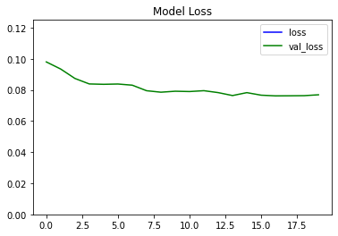
Figure 5. Training Loss Curve for Siamese Network.

From the plotted curves, we see that while the training loss starts near 0.10 and steadily decreases to approximately 0.07, the validation loss similarly trends downward from around 0.11 and remains near 0.08 toward the end of training. This consistent reduction in loss for both sets suggests that the model is effectively learning to distinguish between similar and dissimilar images, while also generalizing reasonably well to unseen data. ![test`1.png](test%601.png) ![test2.png](test2.png)

Figure 6. Model Prediction in Test Data.

The final testing results, as depicted in the figure, highlight a stable decline in both training and validation losses, confirming a robust capability for the model to generalize effectively on unseen data with accuracy of 89.1%.--DIVIDER--# Conclusion Our experiment demonstrated that a Multilayer Perceptron (MLP)–based Siamese network can achieve robust performance in image similarity tasks, as reflected by a validation accuracy of about 0.899 and a test accuracy of approximately 0.891. The steadily decreasing training and validation losses shown in Figure 1 confirm that the network learned effectively without signs of severe overfitting, consistent with best practices for evaluating how well a model generalizes further increase accuracy, exploring new strategies—such as applying more sophisticated data augmentation, expanding the training dataset, and experimenting with deeper MLP architectures—may provide additional performance gains. Integrating advanced preprocessing steps or adopting regularization techniques like batch normalization are also promising avenues for improving model robustness. Looking ahead, future research can explore extending this approach to larger and more diverse datasets, incorporating attention or transformer-based layers, and examining transfer learning methods. By expanding the scope of experimentation, the refined techniques could yield even better results, support real-time recommendation systems, and propel further innovations in fashion item similarity tasks --DIVIDER--# References 1. Nag, R. (2022a, November 19). A comprehensive guide to siamese neural networks. Medium. https://medium.com/@rinkinag24/a-comprehensive-guide-to-siamese-neural-networks-3358658c0513 2. Nag, R. (2022b, November 19). A comprehensive guide to siamese neural networks. Medium. https://medium.com/@rinkinag24/a-comprehensive-guide-to-siamese-neural-networks-3358658c0513