
As we delve into the intricacies of the LLaMA (Large Language Model Meta AI) architecture, it’s crucial to build upon foundational knowledge of the Vanilla Transformer model.
To ensure a comprehensive understanding of LLaMA, I recommend that you first review the concepts of the Vanilla Transformer as discussed in my previous articles. These articles cover essential topics such as self-attention, multi-head attention, positional encoding, and the overall architecture of the Vanilla Transformer. A solid grasp of these concepts will provide a valuable framework for appreciating the enhancements and novel features introduced by LLaMA.
Article on Transformer :- Mastering Transformer
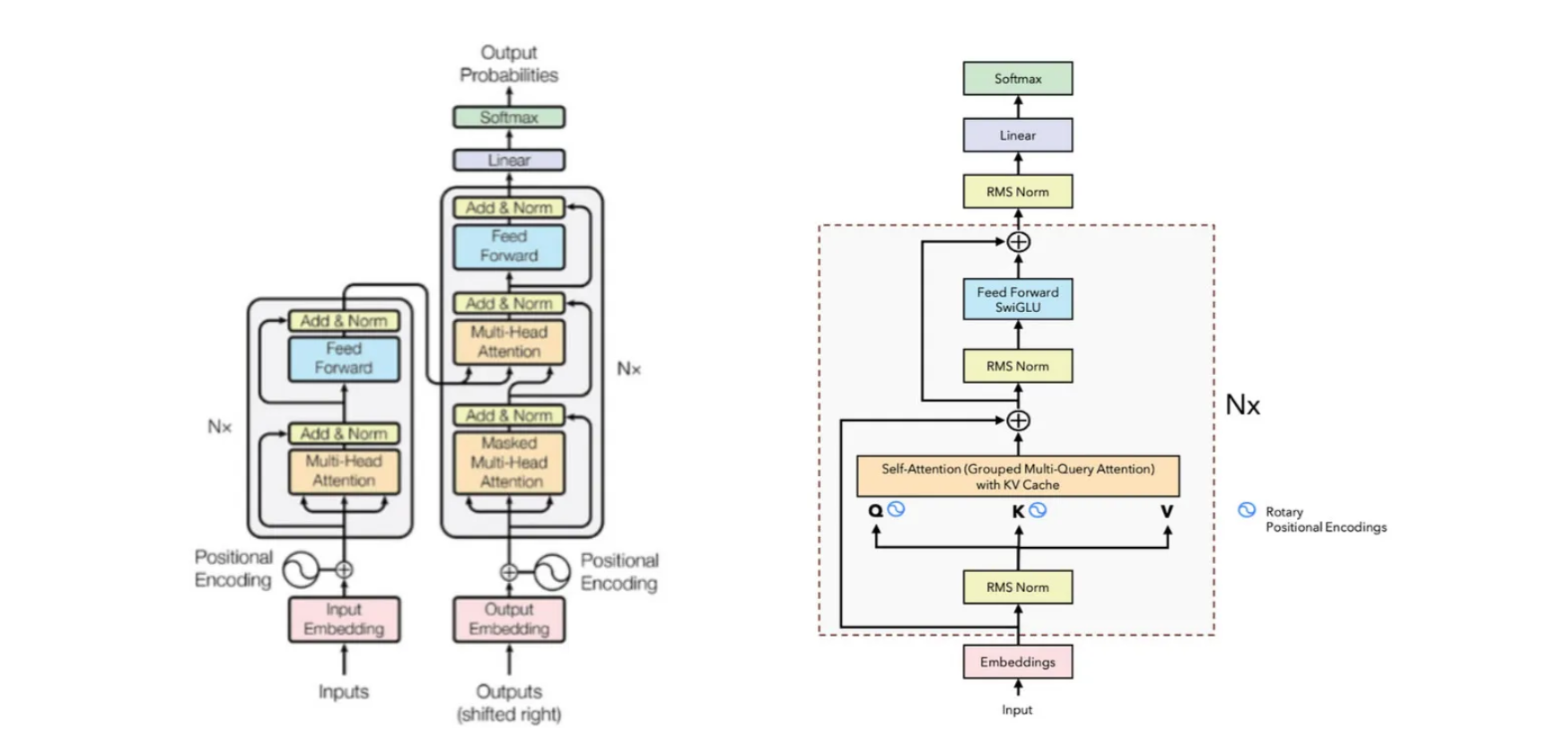
In LLaMA, we utilize only the decoder part of the Vanilla Transformer since it is a Large Language Model trained on the next token prediction task. Therefore, we only need self-attention to predict the next token. Unlike the Vanilla Transformer, which uses positional encoding directly after the input embeddings, LLaMA incorporates RMS Normalization at this stage.
In the Vanilla Transformer, normalization occurs after every block, but in LLaMA, normalization is applied beforehand. Following normalization, we compute the Q (Query), K (Key), and V (Value) matrices for self-attention. The positional encoding in LLaMA has been replaced by Rotary Positional Encodings, which are applied only to the Q and K matrices.
Furthermore, LLaMA’s self-attention mechanism employs KV Cache and Grouped Multi-Query Attention to enhance performance and efficiency. In the Feed Forward layer instead of ReLU, SwiGLU is used.

This image is taken from LLaMA2 paper. LLaMA 1 & LLaMA 2
LLaMA 1 was released in February 2023, featuring four versions with 6.7B, 13B, 32.5B, and 65.2B parameters. The dimension indicates the size of the embeddings. Additionally, each model specifies the number of attention heads, the number of layers, the learning rate, the batch size, and the number of tokens they were trained on.
In LLaMA 2, most model parameters have been doubled. The context length, which refers to the sequence length, has also been extended. The GQA column indicates which models utilize Grouped Query Attention.

Similar to the Transformer, LLaMA uses Byte Pair Encoding (BPE) for tokenization instead of space-based tokenization. Each token is mapped to a unique ID within the vocabulary. These input IDs are then transformed into vectors of size 4096 (compared to 512 in the Transformer). These embeddings are learnable parameters.

The above image show the maths behind nn.Linear(in_features=3, out_features=6, bias=True. This will create matrix W and b. If we input X (6,3) and output O (6,4). The bias vector will be broadcasted to every row in the XWᵀ matrix. After this we apply an actiation function on each item of the matrix O.
The output of a neuron for a given data item depends on the features of the input data and the neuron’s parameters. We can consider the input to a neuron as the output from the previous layer. If the previous layer drastically changes its output after its weights are updated due to gradient descent, the next layer will receive significantly altered inputs. Consequently, the next layer will be forced to drastically readjust its weights in the subsequent step of gradient descent.
The phenomenon where the distributions of internal nodes (neurons) in a neural network change is known as Internal Covariate Shift. This shift is undesirable because it slows down the training process, as neurons must drastically readjust their weights due to significant changes in the outputs of previous layers.

Each item is updated with its normalized value, transforming it into a normal distribution with a mean of 0 and a variance of 1. The parameters gamma and beta are learnable parameters that enable the model to adjust the scale and translation of each feature according to the requirements of the loss function.
With batch normalization we normalize by columns (features)
With layer normalization we normalize by rows (data items)
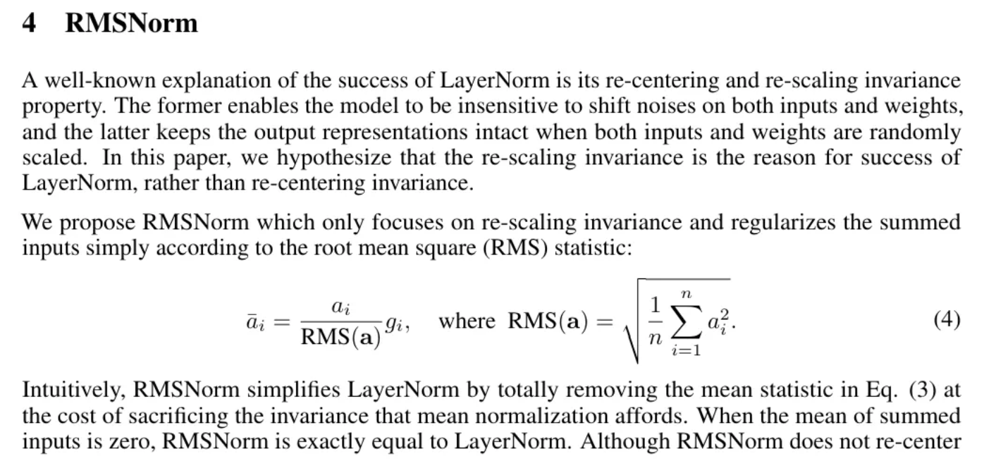
This image is taken from RMS Norm Paper
NOTE that just like layer normalization we also have learnable parameter gamma (g) that is multiplied by the normalization values.
RMS requires less computation compared to Layer Norm.

Absolute positional encodings are fixed vectors added to a token’s embedding to represent its absolute position in a sentence, handling one token at a time. This can be likened to a (latitude, longitude) pair on a map, where each point on Earth has a unique pair.
Relative positional encodings, on the other hand, handle two tokens at a time and are used when calculating attention. Since the attention mechanism captures the “intensity” of the relationship between two words, relative positional encodings inform the attention mechanism about the distance between the two words involved. Given two tokens, a vector representing their distance is created. Relative Positional Encodings was introduced in this paper. We can see in the formula that we are adding the distance ‘a’ between i and j.
Rotatory Positional Embeddings :- The dot product used in the attention mechanism is a type of inner product, which can be thought of as a generalization of the dot product.
Can we find an inner product between the two vectors Q and K used in the attention mechanism that depends only on the two vectors and the relative distance of the tokens they represent?

In the image m and n is the position of the first and second words in the sentence. We can define a function g like the following that only depends on the two embeddings vectors Q and K and their relative distance.

We take the Q and K vectors, multiply them with W (weights) and convert them into complex numbers. Then if we compute the g vector, it will only depend upon the distance of the two vectors (m-n). Now to apply this method on matrics we will use Euler’s formula.

The first matrix in the above expression signifies rotation, if we want to rotate any vector by an angle of θ, we can multiply it with this matrix. So the tokens are rotated now, if two tokens are similar they will have similar rotation. Hence it is called Rotatory Positional Embeddings.
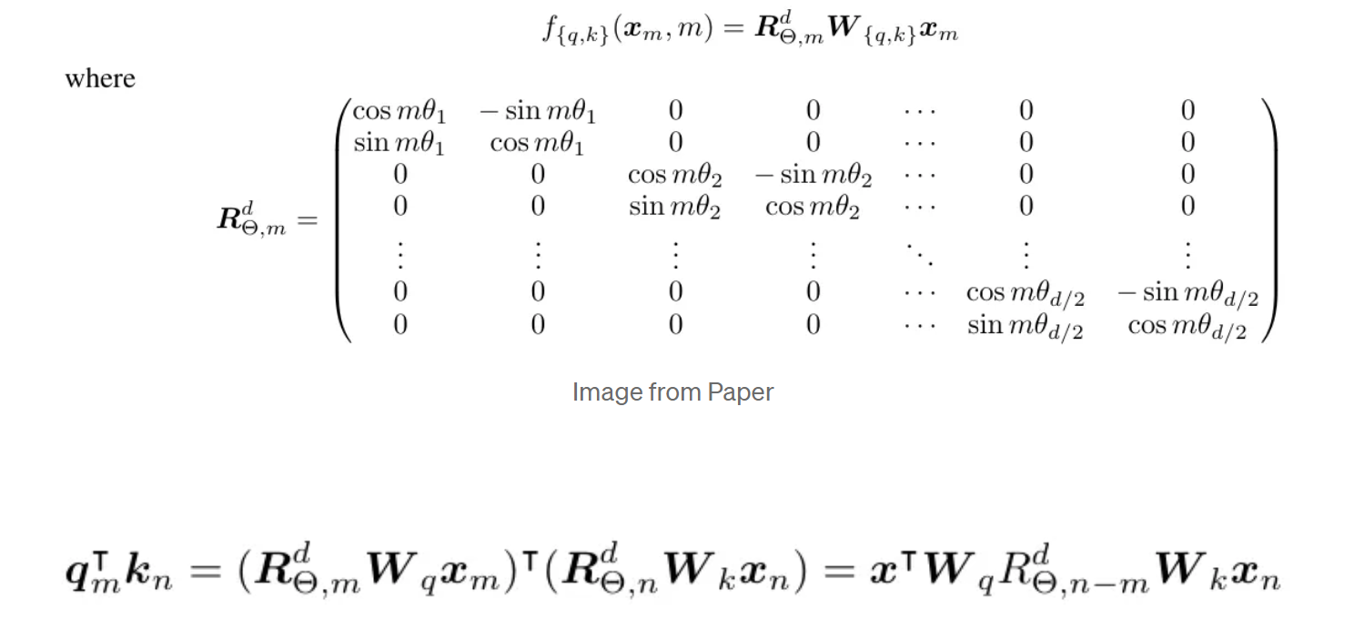
To calculate rotatory positional embeddings using PyTorch we need to create a matrix as shown above. Since this matrix is sparse, it is not convenient to use it due to the high computational requirements.
So the Authors proposed another form which is convenient. Given a token with embedding vector x, and the position m of the token inside the sentence, this is how we compute the position embeddings for the token.

We take the token vector as X and multilpy it element-wise with the cos matrix and then add same vector with positions and sign changed. So in the second position we have x₂ with negative sign and in first position we have x₁ with positive sign. And then we multiply this with the sine matrix.
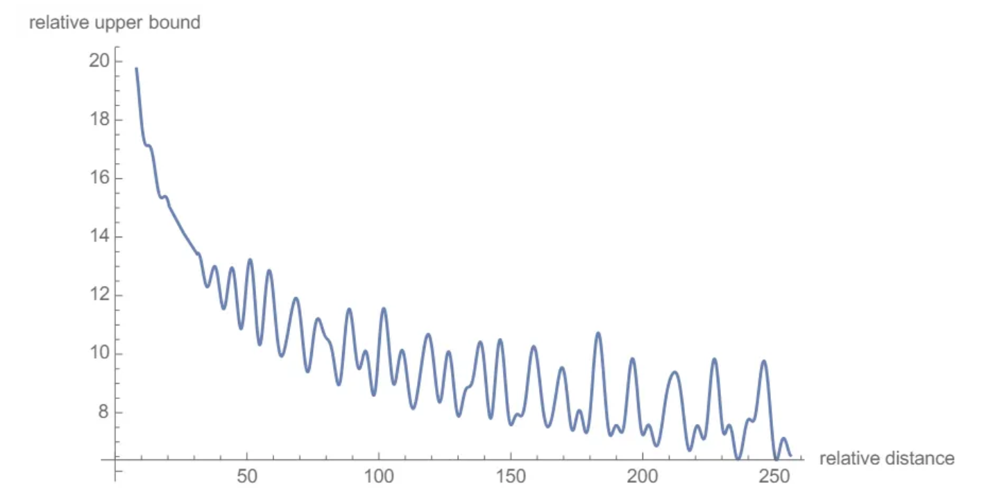
Another interesting aspect is Long-Term Decay. The authors calculated an upper bound for the inner product by varying the distance between two tokens and demonstrated that it decreases as the relative distance increases. This means that the “intensity” of the relationship between two tokens encoded with rotary positional embeddings will be numerically smaller as the distance between them grows.
Rotary position embeddings are applied only to the query and key vectors, not the values. These embeddings are applied after the Q and K vectors have been multiplied by the Q matrix in the attention mechanism, whereas in the vanilla transformer, they are applied before this multiplication.
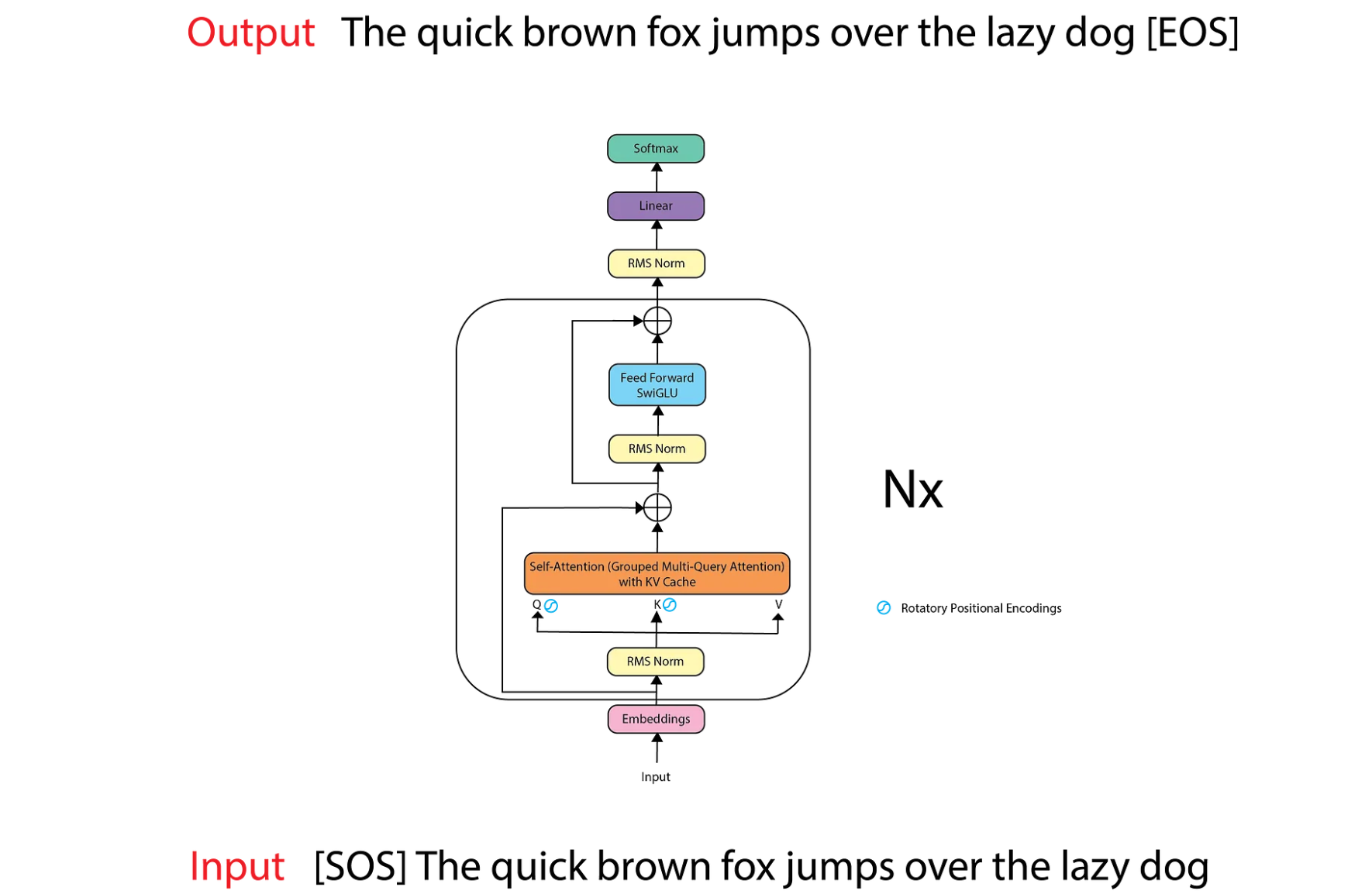
LLaMA is trained on the next token prediction task, meaning that given a sequence, it tries to predict the next most likely token. During training, the input to the model is structured in such a way that the first token is a start of sentence (SOS) token, and the target/output is structured with an end of sentence (EOS) token appended at the end. This setup allows the model to map each input token to the corresponding output token, ensuring that the first token of the input sequence aligns with the first token of the output sequence.
However, this approach poses a problem during inference. While generating predictions, we are only interested in the last token output by the model, as we already have the previous tokens. Nevertheless, the model needs access to all the previous tokens to make its predictions, as they form the context or prompt for each token generation step.
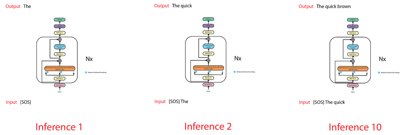
For example, to predict the token “dog,” the model needs to see all the input tokens. This becomes inefficient because, as a sequence-to-sequence model, it will produce the entire sequence, even though we only care about the last token. This leads to unnecessary computations, as the model generates tokens that we already have from previous time steps.
To solve the above problem the authors implemented the KV cache method. KV cache reduces computational redundancy during inference by storing and reusing computations for tokens that have been encountered before.
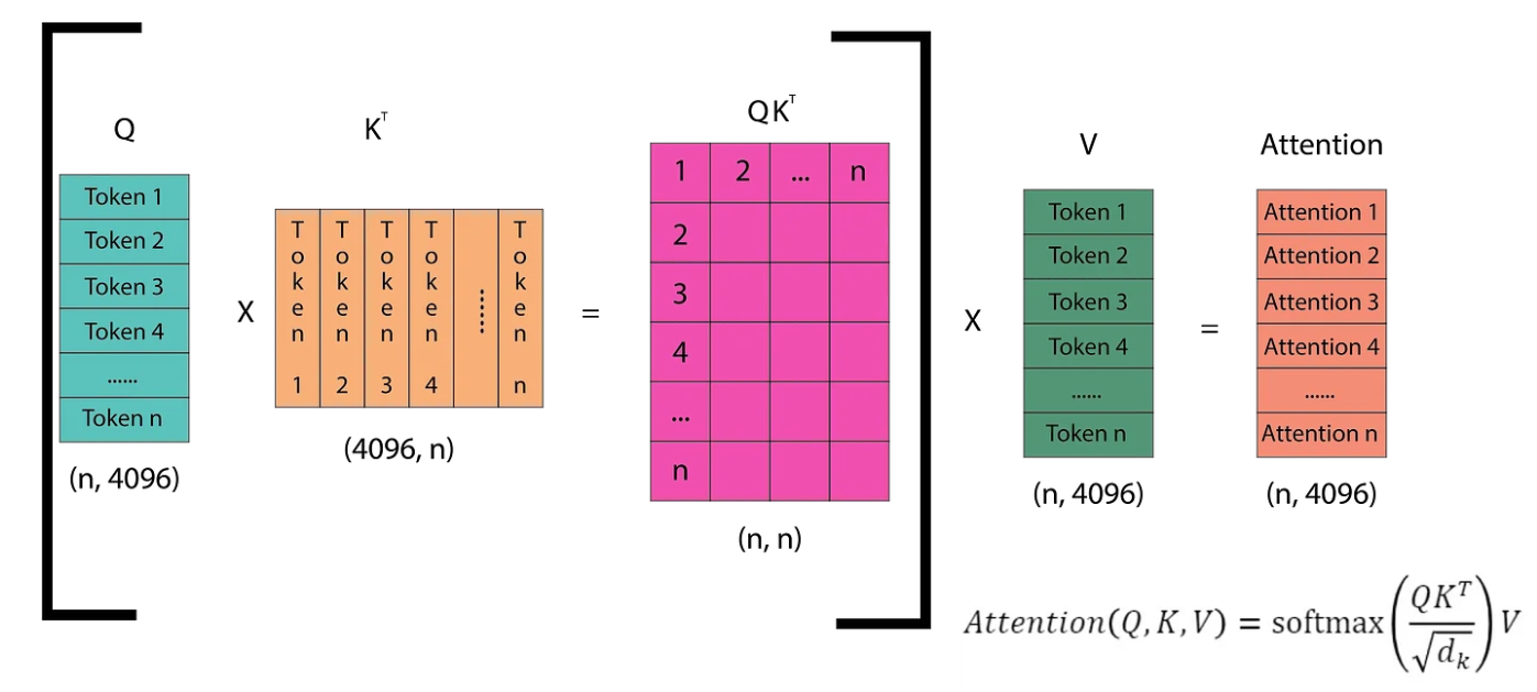
The diagram illustrates how self-attention operates in the next token prediction task. The Q (query) matrix consists of vectors representing each of the n tokens in the sequence. The Kᵀ matrix is the transpose of the Q matrix. Multiplying Q by Kᵀ yields an (n, n) matrix, which is then multiplied by the V matrix to compute the attention scores. These scores are then passed through the linear layers of the Transformer. The linear layers produce logits, which are then fed into the softmax function. Softmax helps determine the token from the vocabulary that the model predicts as the next token. Let’s dive into this step by step.
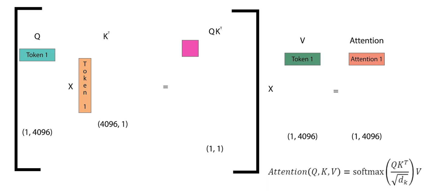
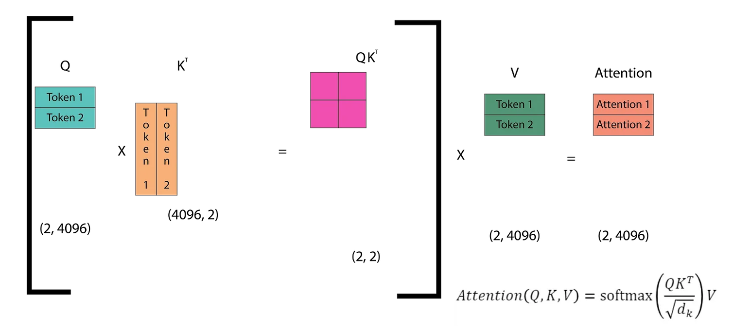
In the first inference step, we only have one token (SOS), which means the Q matrix is of size (1, 4096). Correspondingly, we obtain the first token of the attention matrix (The). In the second inference step, we have two input tokens ([SOS] The) and we get two output tokens (The quick).
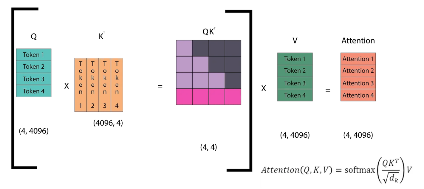
An image of the fourth inference step is shown, where we can observe that we have already computed the dot products of the lower triangle (light purple region)of the QKᵀ matrix. However, in every step, we have to re-calculate these dot products. Since the model is causal, we only need the attention of a token with the tokens before it, not with its successors. Therefore, we just need the last row of the QKᵀ matrix.
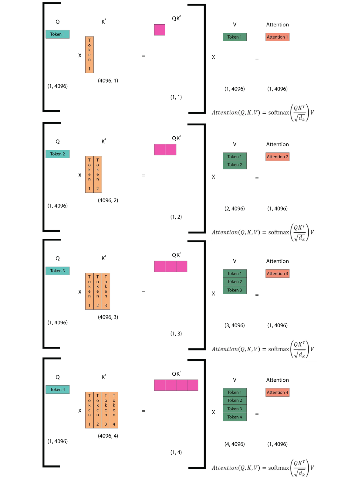
By using the KV cache, we store the K (key) and V (value) matrices. When a new token is encountered, we append it to the cached K and V matrices, while the Q (query) matrix consists only of the output from the previous step. This means that in the second inference step, we do not append the first token to the Q matrix; instead, we replace the first token with the next token. Importantly, we do not take the output of the attention mechanism as input for the next step. Instead, we take the token to which the attention mechanism maps as the input for the next step. This approach reduces redundant computations and improves efficiency during inference.
GPUs excel at performing computations rapidly, but they are not as efficient when it comes to transferring data from their memory. This means that the bottleneck in processing speed is often not the number of operations we perform, but rather the amount of data transfer required by these operations. The size and quantity of tensors involved in calculations heavily influence this data transfer. Therefore, our goal should be to not only optimize the number of operations we perform but also to minimize the memory accesses and transfers.
In the paper on Multi-Query Attention, the author calculates both the number of arithmetic operations performed and the total memory involved in these operations. They find that the number of arithmetic operations performed is O(bnd²), where b is the batch size, n is the sequence length, and d is the size of the embedding vector.
The total memory involved in the operation is given by the sum of all the tensors involved in the calculations, including derived ones, resulting in O(bnd + bn² + d²).
The ratio of total memory to the number of arithmetic operations is
O(1/k + 1/bn). Since this ratio is much smaller than one, it indicates that the number of memory accesses is significantly less than the number of arithmetic operations. Therefore, memory access is not the bottleneck in this case.
When we introduce the KV cache method, the number of arithmetic operations performed remains O(bnd²). However, the total memory involved in the operation changes to O(bn²d + nd²). The ratio of total memory to the number of arithmetic operations then becomes
O(n/d + 1/b).
If the sequence length is close to the size of the embedding vector (n≈d) or the batch size is close to 1 (d≈1), this ratio approaches 1. In such cases, memory access becomes the bottleneck of the algorithm. Typically, the batch size is more than 1, so this is not a significant issue. However, for the n/d term, we need to reduce the sequence length to mitigate the bottleneck.
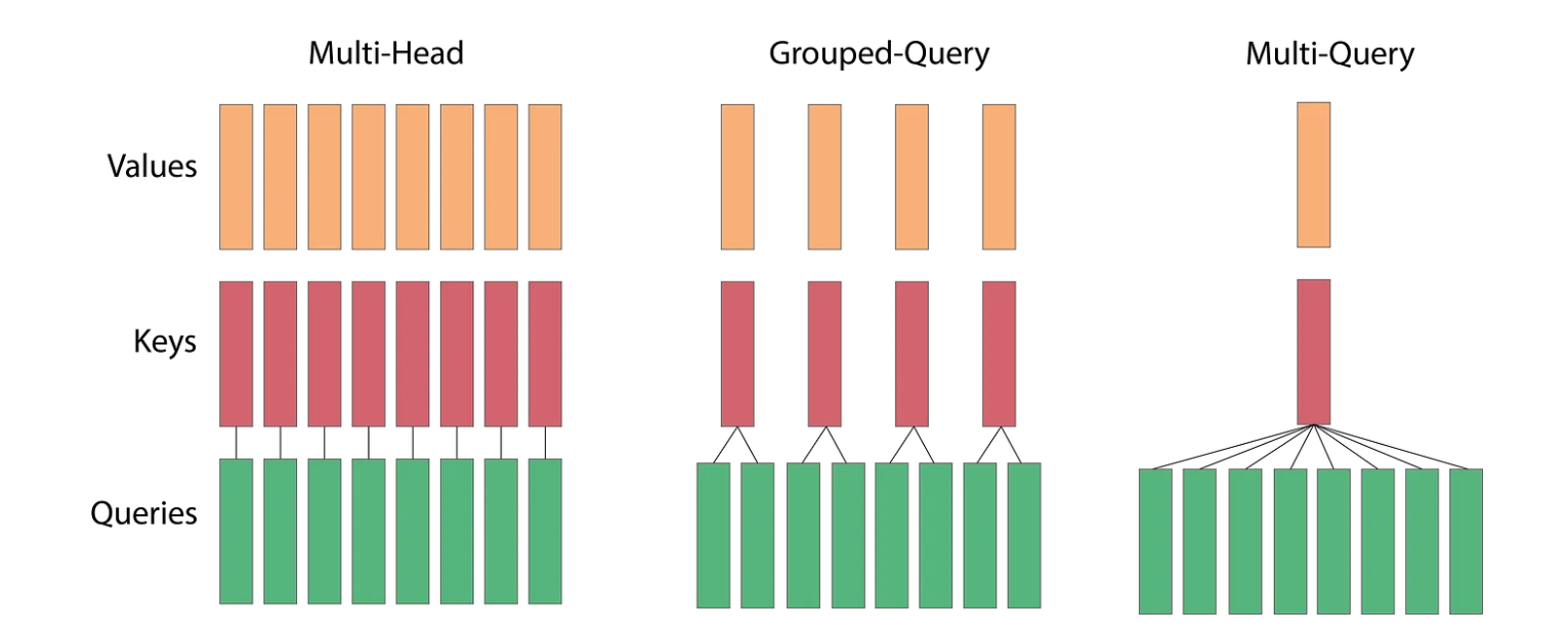
To address this issue, we introduce Multi-query attention with KV cache. This approach removes the h dimension from the K and V matrices while retaining it for Q, meaning all different query heads share the same keys and values.
With this method, the number of arithmetic operations performed remains O(bnd²). However, the total memory involved in the operation changes to O(bnd + bn²k + nd²), and the ratio becomes O(1/d + n/dh + 1/b). Compared to the previous approach, we have reduced the n/d term by a factor of h. This optimization provides significant performance gains while only slightly degrading the model’s quality.
We have multiple heads for the queries but only one head for the keys and values. With grouped multi-head attention, we divide the queries into groups, and each group has a different head for K and V. This reduces the amount of computation required, and although it slightly affects the quality, the decrease is minimal.
The activation function in the feed forward layers is replaced with the SwiGLU activation function. The author compared the performance of a transformer model using different activation functions in the feed forward layer of the transformer architecture. In this modified architecture, there are three matrices instead of the original two. To ensure a fair comparison, the author reduced the dimensions so that the total number of parameters remained the same.
This article discusses the LLaMA model, which enhances the transformer architecture for next token prediction. Key features include Rotary Positional Embeddings, the KV cache method, and Multi-Query Attention, which optimize efficiency and performance. Differences in normalization, activation functions, and the use of SwiGLU are highlighted, emphasizing the importance of these features in improving training speed and handling long-term dependencies.
Next Article :- Building LLaMA from Scratch