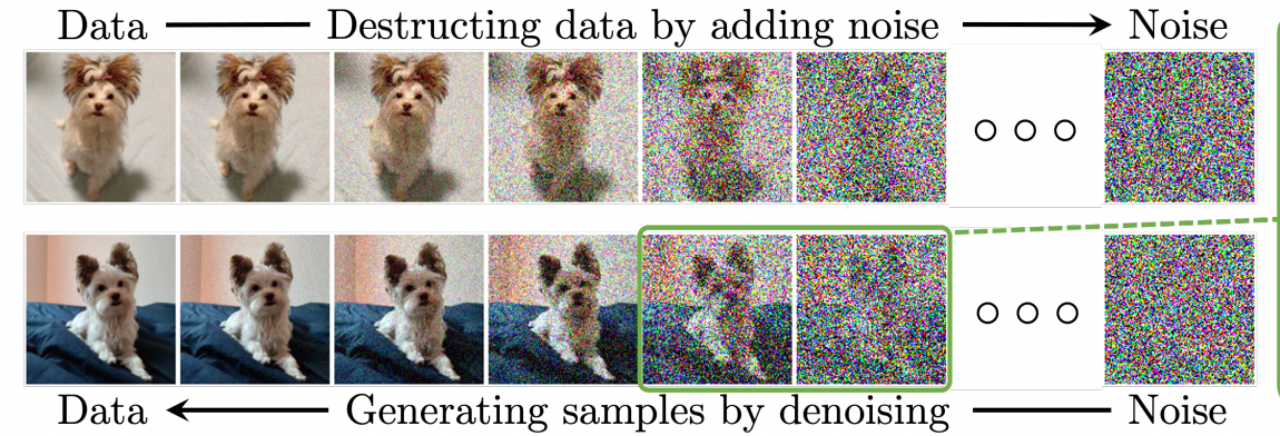
The diffusion model operates by gradually degrading the information in an image through a series of time steps T (x₀, xₜ). At each step, a small amount of Gaussian noise is added, ultimately transforming the image into pure random noise, resembling a sample from a normal distribution, this is known as the forward process. The transition from xₜ₋₁ to xₜ follows this noise-adding mechanism.
To reverse this, a neural network is trained to progressively remove the noise, step by step. Once trained, the model can start with random noise drawn from a normal distribution. It iteratively denoises the input, each pass removing a bit more noise, until the final result is a clear image that resembles the original distribution.
This approach parallels variational autoencoders (VAEs) in concept. In VAEs, an image is encoded into the mean and variance of a Gaussian distribution, and a decoder then reconstructs the image by sampling from this distribution. Similarly, the diffusion model’s denoising process transforms random noise back into coherent images, analogous to the reconstruction phase in VAEs.
Diffusion refers to the movement of molecules from areas of higher concentration to lower concentration. In a statistical sense, a diffusion process is a stochastic Markov process characterized by continuous sample paths. Stochastic implies the presence of randomness, while Markov indicates that the future state depends only on the current state — knowledge of past states adds no further information. Continuous means the process evolves smoothly, without sudden jumps.
In statistics, diffusion describes the transformation of a complex distribution into a simpler one, typically a prior distribution, within the same domain. If certain conditions are met, repeatedly applying a transition kernel to samples from any distribution will eventually yield samples from this simpler prior. In the case of diffusion models, the input image represents a complex distribution, which is progressively transformed into a simple normal distribution.

let’s assume the coefficient to be as ⍺ and ꞵ, both independent to each other. We will start with the distribution given at left and we will sample the image and chart the histogram plot. Then we will apply the transition step once (⍺=0.5, ꞵ=0.1) which will lead to change in the values and hence change in the histogram plot.
By applying the equation once, we observe a gradual transition from the original state to a more random state. With ⍺ = 0 and ꞵ = 1, we immediately obtain a Gaussian distribution. However, the goal is to achieve this transformation progressively through incremental changes, which defines the diffusion process. If ⍺ > 1, the variance would increase uncontrollably, preventing convergence to the desired distribution. Thus, some decay in the original values is essential. A suitable choice is ⍺ = 0.999, just below 1.
Next, the noise term ꞵ must be introduced gradually. High values of ꞵ would cause abrupt changes in the distribution, which we want to avoid. Instead, the transformation should occur slowly, ensuring that as the original distribution is degraded, it increasingly resembles a normal distribution. Ultimately, we arrive at the optimal values of ⍺ = √0.99 and ꞵ = √0.01.
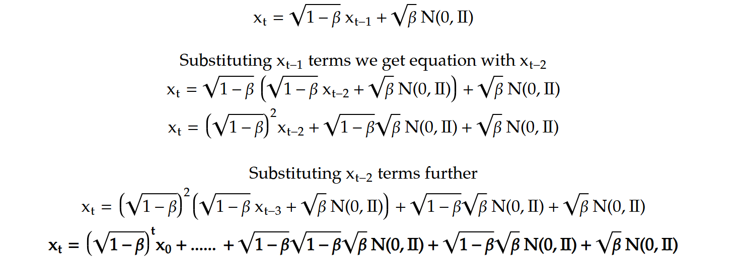
Mathematically, substituting the terms xₜ₋₁ and xₜ₋₂ into the equation reveals a repetitive pattern in the process, reinforcing the gradual nature of the transformation.
For all time steps, we ultimately derive a final equation where only the first term contains x₀. As T becomes sufficiently large, this first term approaches zero since all the values in the product are less than 1. The remaining terms are Gaussian distributions with a mean of 0 but different variances.
Since these terms are independent, they can be combined into a single Gaussian distribution, with the overall mean still being 0 and the variance equal to the sum of the individual variances. Specifically, the last term will have a variance of β, the second-to-last will have β(1−β), and so forth. This forms a geometric progression (GP) where the first term is β and the common ratio is 1−β. Therefore, the sum over T terms can be expressed as: β(1−(1−β)ₜ) / (1−(1−β)) ~ β/β = 1
We are essentially linking the extent to which the original distribution’s structure is destroyed to the amount of noise we introduce. The diffusion process is discretized into finite steps for a 1D distribution. This approach can be extended to a w×h, where the output of the forward process is a w×h, with each pixel resembling a sample from a Gaussian distribution with a mean of 0 and a variance of 1.
In practice, instead of using a constant noise variance at each step, a schedule is applied. The authors propose a linear schedule that gradually increases the noise variance over time. This strategy is logical because, at the beginning of the reverse process, the model needs to learn to make larger adjustments. As it nears a clear image, smaller, more refined adjustments are required.
This schedule ensures that the variance scales smoothly from the input distribution to the target Gaussian. With a fixed noise variance, the reduction in distribution variance is significant early on and reaches nearly 1 after around 500 steps. However, when following the suggested schedule, the variance reduction is more gradual and consistent over a larger portion of the time steps, resulting in a smoother transition.
To get the value of X at t=1000, we need to apply the transition 1000 times to go through the entire markov chain which is not efficient.
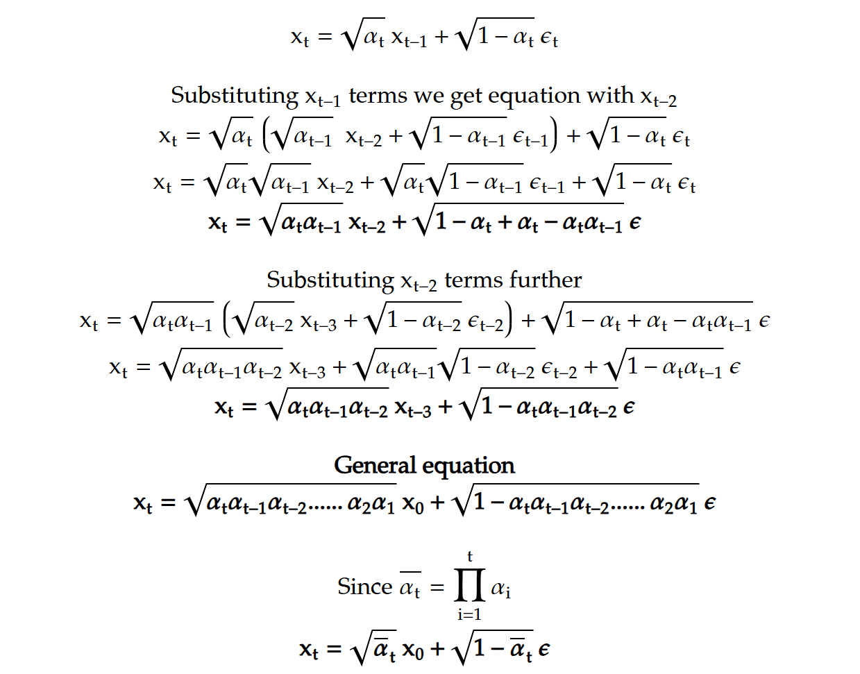
We need to do this entire maths just for noising the input image, the reverse process is also a markov chain with gaussian transition probability. We can’t compute it directly because for that we need to compute the entire data distribution however we can approximate it by a distribution P, which is formulated as a gaussian whose mean and variance are the parameters that we are interested in learning.

We have a similar situation in VAE, where we don’t know the true distribution of X given Z but we learn to approximate it by neural network. so we want to learn P(X | Z) such that we are able to generate images as close to our training data distribution as possible.
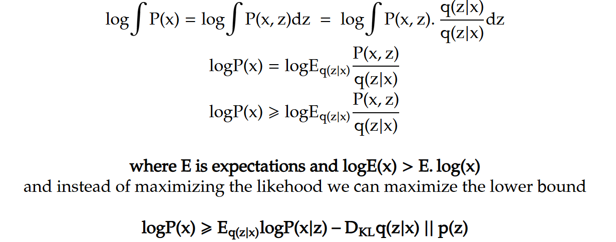
The first term, assuming P follows a Gaussian distribution, becomes the reconstruction loss between the generated output and the ground truth image. The second term represents the KL divergence between our prior — a Gaussian distribution with a mean of zero and unit variance — and the distribution predicted by the encoder. This concept can be extended to the diffusion process.
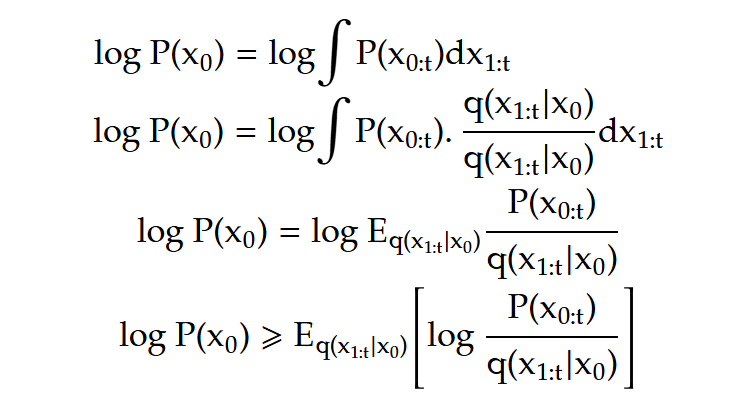
In this case, rather than transitioning directly to Zₜ, we move gradually through a sequence of latent variables from x₁ to xₜ. Here, q(z ∣ x) is replaced by q(xₜ ∣ xₜ₋₁), which is fixed and not learned. As before, the objective is to maximize the likelihood of the observed data.
Term inside expectation, q is the forward process and P is the approximation of the reverse process. Since the chain is Markov, q(xₜ ∣ xₜ₋₁) = q(xₜ ∣ xₜ₋₁, x₀).
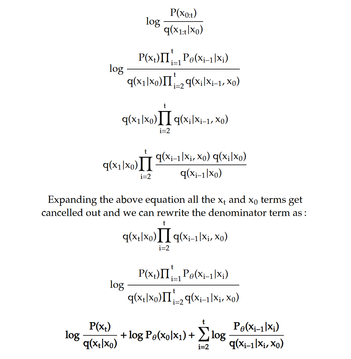
Let’s look at the denominator, we can apply bayes theorem to get this:
With the remaining terms we put that together in the lower bound equation, we can separate this equation as a sum of three log terms. Remember all of this was under the expectation of Q.
The first term is like KL divergence prior term but here because we are using diffusion q is fixed and the final q(xₜ ∣ x₀) according to theory will actually be very close to normal distribution, so this is parameter free and we won’t bother optimizing this. Second term is the reconstruction of our input x₀ given x₁ and the last term is the sum of quantities which are nothing but KL divergence. And since we want to maximize the lower bound we want to minimize all of these scale terms the good part about this formulation is that the last term involves two quantities of same form and this is simply requiring the approximate denoising transition distribution to be very close to the ground truth denoising transition distribution conditioned on x₀.
Instead of q(xₜ₋₁ ∣ xₜ) we now have q(xₜ₋₁ ∣ xₜ, x₀), which is conceptually easier to compute. By applying Bayes’ theorem, we can break this down. Each term in this process is Gaussian, and we have already derived the necessary expressions. The first term represents the forward process, and although it is conditioned on x₀, it remains unaffected because the forward process follows a Markov chain.
The other two terms can be expressed using the recursion established earlier, allowing us to transition from x₀ to a noisy image at any time step t. Since these terms are Gaussian, they can be represented in exponential form. The primary objective is to compute xₜ₋₁. To achieve this, we can rewrite the expression into a perfect square, enabling us to derive the equation for a Gaussian distribution. With this approach, we separate the x²ₜ₋₁ terms, the xₜ₋₁ terms and everything that is independent of xₜ₋₁.
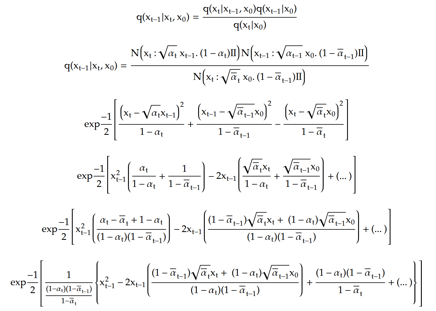
Up to this point, we have expressed the normal distribution in exponential form and simplified it using algebraic summation. Now, we will focus on the final term, which is independent of xₜ₋₁. After further simplification, we find that this term resolves into the square of an expression, multiplied by 2xₜ₋₁.
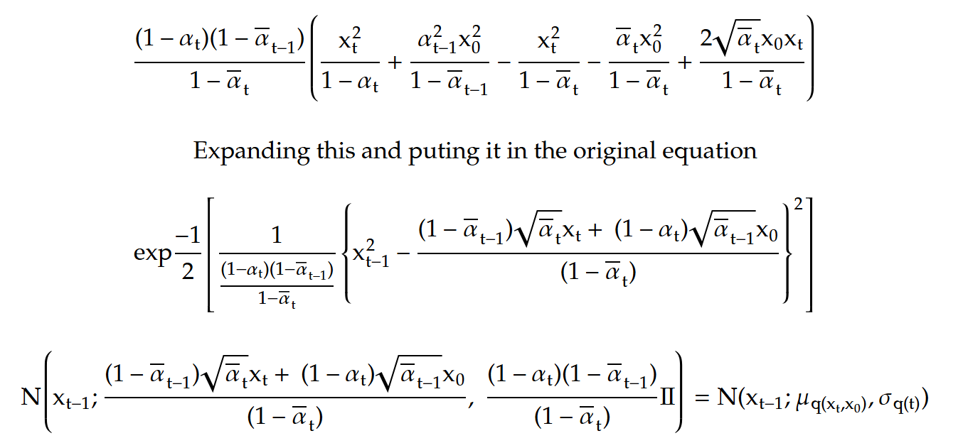
This allows us to write the whole equation for reverse distribution as a gaussian with being the mean and variance. And for the last term we need to compute q(xₜ₋₁ | xₜ₋₁, x₀).
We can see that the mean is the weighted average of xₜ and x₀. If we compute the weight for x₀ then we will see that it is a very low value at higher time steps and as we move closer to the end of the reverse process this weight increases. And from the graph we can see the weight is 0 for a long time but when we plot the log values we can there is indeed an increase overtime.
For the reverse distribution process we have to approximate it because for generation, we won’t really have x₀ but because we know that our reverse is a gaussian we can have our approximation also as a gaussian. And all we need to do is learn the mean and variance. The first thing that the authors do is fix the variance to be exactly the same as the ground truth denoising step.
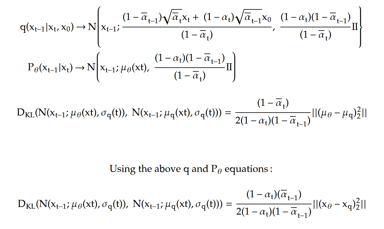
The likelihood function, all the terms are as the expectation of q making it KL divergence and when we use the KL divergence formula for gaussian because here both the distributions have the exact same variance it will end up being the square of difference between the means divide the twice the variance which is this quantity so since our goal is to maximize the likelihood we need to reduce the difference now because our ground truth denoising step has mean.
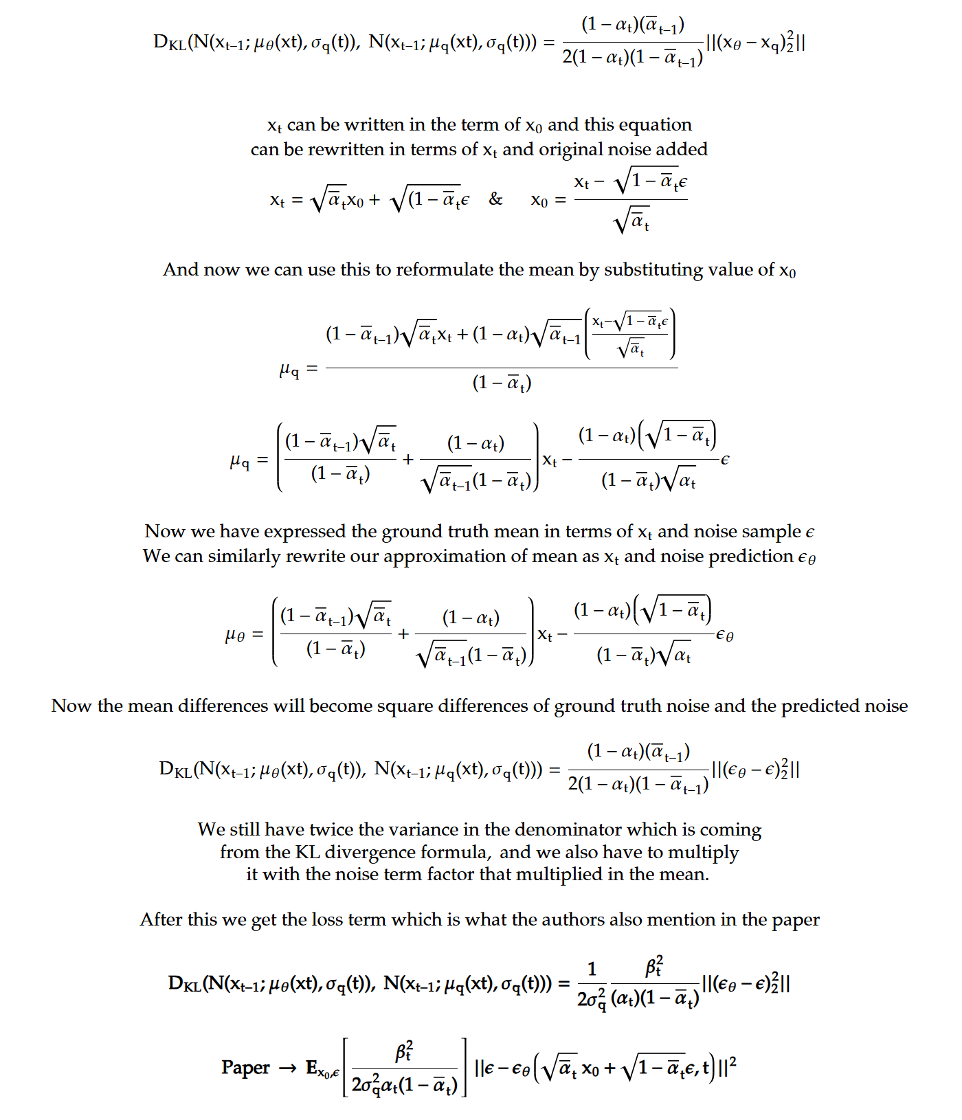
Recap → in the likehood term we ignored the first term and focused on the last summation term. We identified that it can be written as Scaled Squared Difference between the ground truth noise and the noise prediction generated by some model using xₜ as input, in practice we also provide time step as well. The authors actually ignored the scaling altogether and through experiments find that on just training the model on the Square Difference of Noise is good enough.
The second term in the likehood is wrapped under this loss by having the model approximate the noise that was to x₀ to get x₁.
During training, we first sample an image from our dataset and select a time step t uniformly. Next, we sample random noise from a normal distribution. Using the equation for xₜ in terms of x₀ and ϵ, we obtain the noisy version of the image at time step t within the diffusion process. We then use the original image, the sampled noise, the time step, and the noise schedule to compute the cumulative product terms. This noisy image is passed through the neural network, and we train the network using a loss function to minimize the difference between the predicted noise and the actual noise. By training over many steps, we cover all time steps and effectively optimize each component of the summation term.
For image generation, we follow the reverse process by iteratively sampling from the denoising step distribution P that our neural network has learned. To generate an image, we begin with a random sample from a normal distribution as the initial image at step t. This is then passed through our trained model to predict the noise. To clarify, our approximate denoising distribution is defined by the mean of the noisy image at time step t and the predicted noise.
Once we have the predicted noise, we can sample an image from the distribution using the mean image and the variance, which was fixed to be the same as in the forward process. This sampled image becomes our xₜ₋₁. We continue repeating this process until we arrive at the original image x₀. The only variation is that, to go from x1 to x₀, we directly return the mean image.