Implementing Multiple Linear Regression from Scratch

Overview

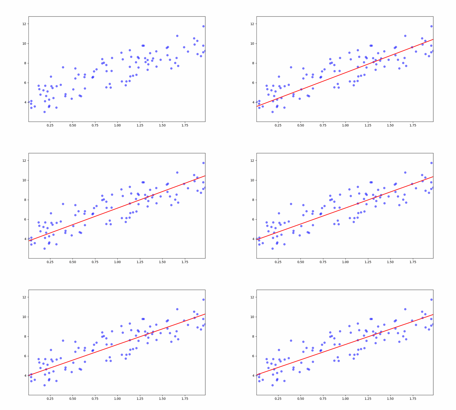
Multiple Linear Regression (MLR) is a statistical method that models the relationship between a dependent variable and multiple independent variables. It extends simple linear regression, which uses a single feature to predict the outcome, to handle multiple features. The general form of the MLR equation is:

Where:

• is the dependent variable (target).
• are the independent variables (features).
• is the intercept (bias).
• are the coefficients (weights) for the features.
• represents the error term (noise).

The goal of multiple linear regression is to estimate the coefficients such that the predicted values are as close as possible to the actual values.

Approach

We'll implement multiple linear regression from scratch using two different methods:

1. Gradient Descent: An iterative approach to optimize the model parameters.
2. Normal Equation: A direct mathematical solution to compute the optimal parameters.

1. Data Generation and Preprocessing

To demonstrate the MLR model, we first generate synthetic data. For this example, we will create a dataset with three features, where the true relationship is:

The noise is added to simulate real-world data variability, making it more challenging for the model to fit the data perfectly.

2. Building the Multiple Linear Regression Class

We implement the model using two methods: Gradient Descent and Normal Equation.

Gradient Descent Method

Gradient descent is an optimization algorithm used to minimize the loss function. In the case of linear regression, the loss function is the Mean Squared Error (MSE). Gradient descent iteratively adjusts the model's parameters to find the values that minimize the loss.

import numpy as np

class MultipleLinearRegression:
    def __init__(self, learning_rate=0.01, n_iterations=1000):
        self.learning_rate = learning_rate
        self.n_iterations = n_iterations
        self.weights = None
        self.bias = None
        self.history = {'loss': [], 'weights': [], 'bias': []}
    
    def predict(self, X):
        return np.dot(X, self.weights) + self.bias
    
    def fit(self, X, y):
        n_samples, n_features = X.shape
        self.weights = np.zeros(n_features)
        self.bias = 0
        
        for i in range(self.n_iterations):
            y_predicted = self.predict(X)
            
            # Compute gradients
            dw = (1/n_samples) * np.dot(X.T, (y_predicted - y))
            db = (1/n_samples) * np.sum(y_predicted - y)
            
            # Update parameters
            self.weights -= self.learning_rate * dw
            self.bias -= self.learning_rate * db
            
            # Track loss and parameters
            loss = np.mean((y_predicted - y) ** 2)
            self.history['loss'].append(loss)
            self.history['weights'].append(self.weights.copy())
            self.history['bias'].append(self.bias)

Normal Equation Method

The normal equation provides a closed-form solution to calculate the optimal weights directly. It avoids the need for iterative optimization but can be computationally expensive for large datasets.

Where:

• is the matrix of input features (with a column of ones added for the intercept term).
• is the vector of target values.
• is the vector of coefficients (including the intercept).
• is the transpose of the matrix .
• is the inverse of the matrix .

class MultipleLinearRegressionNormal:
    def __init__(self):
        self.weights = None
        self.bias = None
    
    def predict(self, X):
        return np.dot(X, self.weights) + self.bias
    
    def fit(self, X, y):
        # Add bias term (column of ones) to the feature matrix
        X_b = np.c_[np.ones((X.shape[0], 1)), X]
        
        # Compute the optimal weights using the normal equation
        betas = np.linalg.inv(X_b.T @ X_b) @ X_b.T @ y
        
        # Separate bias and weights
        self.bias = betas[0]
        self.weights = betas[1:]

3. Training the Model

After defining the models, we proceed to train them using the generated synthetic data. The dataset is split into training and testing sets, and the models are fitted to the training data.

# Generate synthetic data
X, y = generate_data()
X_train, X_test, y_train, y_test = train_test_split(X, y, test_size=0.2, random_state=42)

# Scale the features (important for gradient descent)
scaler = StandardScaler()
X_train_scaled = scaler.fit_transform(X_train)
X_test_scaled = scaler.transform(X_test)

# Train Gradient Descent Model
gd_model = MultipleLinearRegression(learning_rate=0.06, n_iterations=700)
gd_model.fit(X_train_scaled, y_train)

# Train Normal Equation Model
normal_model = MultipleLinearRegressionNormal()
normal_model.fit(X_train_scaled, y_train)

4. Evaluating the Model

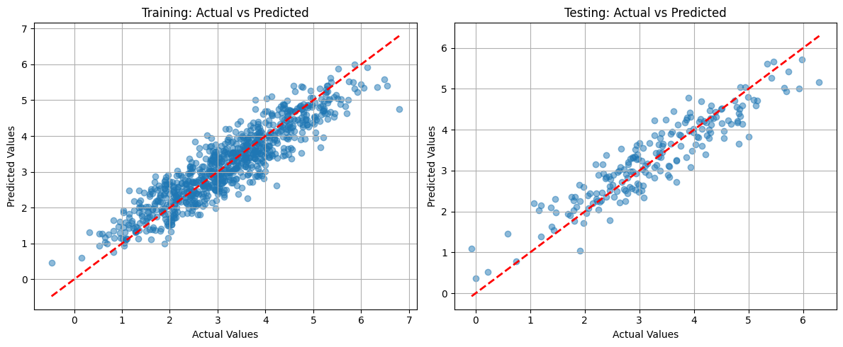
After training, we evaluate both models using the R² score, which measures the proportion of variance explained by the model. A higher R² score indicates a better model fit.

The R² (R-squared), or coefficient of determination, is a statistical measure that indicates how well the independent variables explain the variance in the dependent variable. The formula for R² is:

Where:

• is the actual value of the dependent variable for the sample.
• is the predicted value for the sample.
• is the mean of the actual values.
• is the number of data points.

Interpretation of R²:

• : The model explains 100% of the variance in the dependent variable.
• : The model does not explain any of the variance, and predictions are as good as simply predicting the mean of the target variable.
• : The model is worse than predicting the mean of the target variable, which often happens when the model is poorly fitted.

Steps:

1. Calculate the total sum of squares (TSS): — measures the total variance in the data.
2. Calculate the residual sum of squares (RSS): — measures the variance not explained by the model.
3. R² is the proportion of the variance that is explained by the model, calculated as .

from sklearn.metrics import r2_score

# Evaluate the models
gd_predictions = gd_model.predict(X_test_scaled)
normal_predictions = normal_model.predict(X_test_scaled)

print("Gradient Descent Model R² Score:", r2_score(y_test, gd_predictions))
print("Normal Equation Model R² Score:", r2_score(y_test, normal_predictions))

5. Visualization

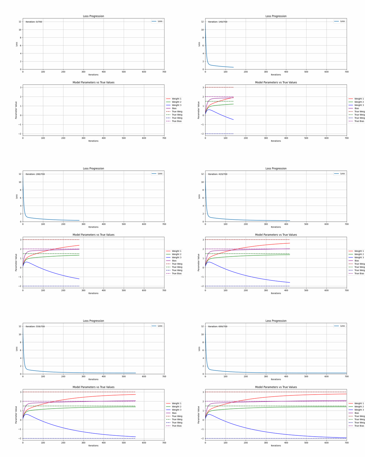
Visualizing the training process can help us understand the model’s convergence. We plot the loss progression over iterations and track how the weights change during training.

import matplotlib.pyplot as plt

# Plot loss progression
plt.figure(figsize=(10, 5))
plt.subplot(1, 2, 1)
plt.plot(gd_model.history['loss'])
plt.title('Loss Progression')
plt.xlabel('Iterations')
plt.ylabel('Mean Squared Error')

# Plot weight changes
plt.subplot(1, 2, 2)
weights_history = np.array(gd_model.history['weights'])
for i in range(weights_history.shape[1]):
    plt.plot(weights_history[:, i], label=f'Weight {i+1}')
plt.title('Weight Progression')
plt.xlabel('Iterations')
plt.ylabel('Weight Value')
plt.legend()

plt.tight_layout()
plt.show()

Complete Example Code

Here’s the complete code combining all steps:

import numpy as np
import matplotlib.pyplot as plt
from sklearn.model_selection import train_test_split
from sklearn.metrics import r2_score
from sklearn.preprocessing import StandardScaler

# Set random seed for reproducibility
np.random.seed(42)

# Generate synthetic data
def generate_data(n_samples=100, n_features=3):
    X = np.random.randn(n_samples, n_features)
    true_coefficients = np.array([3, 1.5, -2])
    noise = np.random.normal(0, 0.5, n_samples)
    y = 2 + np.dot(X, true_coefficients) + noise
    return X, y

# Generate and prepare data
X, y = generate_data()
X_train, X_test, y_train, y_test = train_test_split(X, y, test_size=0.2, random_state=42)

# Scale the features
scaler = StandardScaler()
X_train_scaled = scaler.fit_transform(X_train)
X_test_scaled = scaler.transform(X_test)

# Train Gradient Descent Model
gd_model = MultipleLinearRegression(learning_rate=0.06, n_iterations=700)
gd_model.fit(X_train_scaled, y_train)

# Train Normal Equation Model
normal_model = MultipleLinearRegressionNormal()
normal_model.fit(X_train_scaled, y_train)

# Evaluate models
gd_predictions = gd_model.predict(X_test_scaled)
normal_predictions = normal_model.predict(X_test_scaled)

print("Gradient Descent Model R² Score:", r2_score(y_test, gd_predictions))
print("Normal Equation Model R² Score:", r2_score(y_test, normal_predictions))

# Visualization
plt.figure(figsize=(12, 5))
plt.subplot(1, 2, 1)
plt.plot(gd_model.history['loss'])
plt.title('Loss Progression')
plt.xlabel('Iterations')
plt.ylabel('Mean Squared Error')

plt.subplot(1, 2, 2)
weights_history = np.array(gd_model.history['weights'])
for i in range(weights_history.shape[1]):
    plt.plot(weights_history[:, i], label=f'Weight {i+1}')
plt.title('Weight Progression')
plt.xlabel('Iterations')
plt.ylabel('Weight Value')
plt.legend()

plt.tight_layout()
plt.show()

Conclusion

By implementing multiple linear regression from scratch, we gain a deeper understanding of the underlying mechanics of regression models. The two methods—Gradient Descent and Normal Equation—offer different trade-offs in terms of complexity and computational efficiency. Gradient Descent is more flexible and scales well with large datasets, while the Normal Equation provides a direct solution, making it faster for smaller datasets.

Key Takeaways:

• Multiple Linear Regression models the relationship between multiple features and a target variable.
• Gradient Descent and Normal Equation are two common methods for solving MLR problems.
• Feature scaling is important for

Gradient Descent to converge efficiently.

• Evaluating the model using metrics like R² helps assess its performance.

Potential Improvements:

• Implement regularization (e.g., Lasso, Ridge) to prevent overfitting.
• Use cross-validation to get a better estimate of model performance.
• Explore more advanced optimization algorithms (e.g., Stochastic Gradient Descent).

If you're looking to dive deeper into linear regression and machine learning, here are some great resources:

• Kaggle: Explore the Notebook
• LinkedIn: Connect with me
• GitHub: Explore Repo
• scikit-learn Documentation on Linear Regression

Feel free to reach out with any questions or thoughts. Happy learning and coding!