
In the field of data compression, traditional methods have long dominated, ranging from lossless techniques such as ZIP file compression to lossy techniques like JPEG image compression and MPEG video compression. These methods are typically rule-based, utilizing predefined algorithms to reduce data redundancy and irrelevance to achieve compression. However, with the advent of advanced machine learning techniques, particularly Auto-Encoders, new avenues for data compression have emerged that offer distinct advantages over traditional methods in certain contexts.
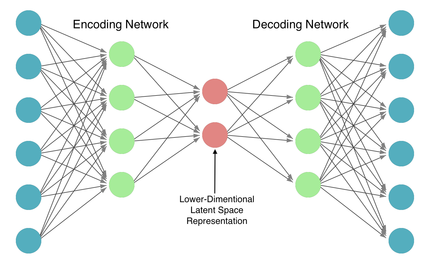
Auto-encoders are a class of neural network designed for unsupervised learning of efficient encodings by compressing input data into a condensed representation and then reconstructing the output from this representation. The primary architecture of an auto-encoder consists of two main components: an encoder and a decoder. The encoder compresses the input into a smaller, dense representation in the latent space, and the decoder reconstructs the input data from this compressed representation as closely as possible to its original form.
The flexibility and learning-based approach of Auto-Encoders provide several benefits over traditional compression methods:
In the notebook included in the Resources section, an experimental framework is set up to investigate the compression capabilities of Auto-Encoders using the MNIST dataset. MNIST, a common benchmark in machine learning, consists of 60,000 grayscale images in 10 classes of size 28x28, providing a diverse range of handwritten digits for evaluating model performance.
For the image compression task, we utilize a convolutional autoencoder, leveraging the spatial hierarchy of convolutional layers to efficiently capture the patterns in image data. The autoencoder's architecture includes multiple convolutional layers in the encoder part to compress the image, and corresponding deconvolutional layers in the decoder part to reconstruct the image. The model is trained with the objective of minimizing the mean squared error (MSE) between the original and reconstructed images, promoting fidelity in the reconstructed outputs.
The notebook details a systematic exploration of different sizes of the latent space, ranging from high-dimensional to low-dimensional representations. The goal is to understand how the dimensionality of the latent space affects both the compression percentage and the quality of the reconstruction. The compression percentage is calculated based on the ratio of the dimensions of the latent space to the original image dimensions, while the reconstruction error is measured using the MSE. We explore 4 scenarios of compression: 50%, 90%, 95% and 99%.
Let's examine a sample of images to visualize how the size reduction in the latent space affects the quality of reconstructed images:
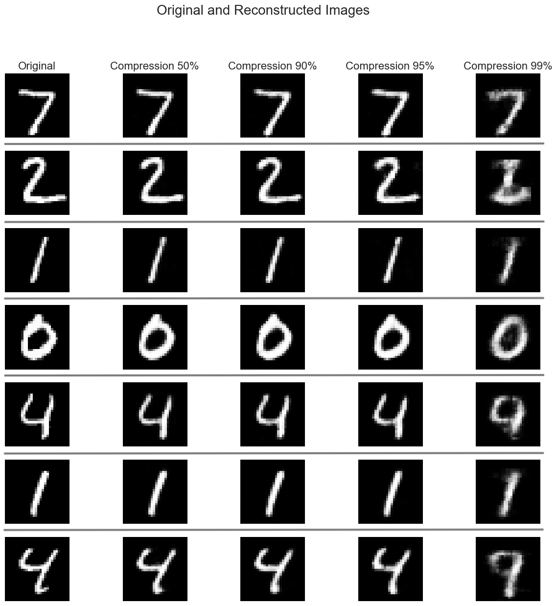
As we increase the compression ratio, we observe:
This highlights the trade-off between compression efficiency and image fidelity.
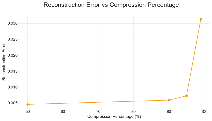
We now examine the relationship between compression ratio and reconstruction loss (MSE). Specifically, as the latent space is reduced, achieving higher compression percentages, the reconstruction error initially remains low, indicating effective compression. However, a marked increase in reconstruction error is observed as the latent dimension is further reduced beyond a certain threshold . This suggests a boundary in the compression capabilities of the autoencoder, beyond which the loss of information significantly impacts the quality of the reconstructed images.
The chart below illustrates the reconstruction error for each digit at 95% and 99% compression rates.
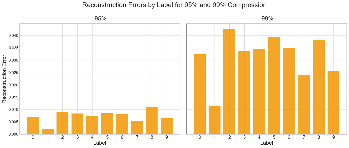
Our analysis reveals that the digit "1" shows the lowest reconstruction error, while digit "2" exhibits the highest error at 95% compression, and digit "8" at 99% compression. However, it's crucial to understand that these results don't account for the total amount of information each digit contains, often visualized as the amount of "ink" or number of pixels used to write it.
The lower error for digit "1" doesn't necessarily mean it's simpler to represent in latent space. Rather, even if all digits were equally complex to encode per unit of information, digits like "2" or "8" would naturally accumulate more total error because they contain more information (more "ink" or active pixels).
For a fairer comparison, we would need to normalize the error by the amount of information in each digit. For instance, if we measured error per 100 pixels of "ink", we might find that the relative complexity of representing each digit in the latent space is more similar than the raw error suggests.
Below is a scatter plot that visualizes the distribution of original images (blue points) and their reconstructed counterparts (red points) using t-SNE. This visualization allows us to compare the high-dimensional structure of the original and reconstructed data in a 2D space.
Key observations:
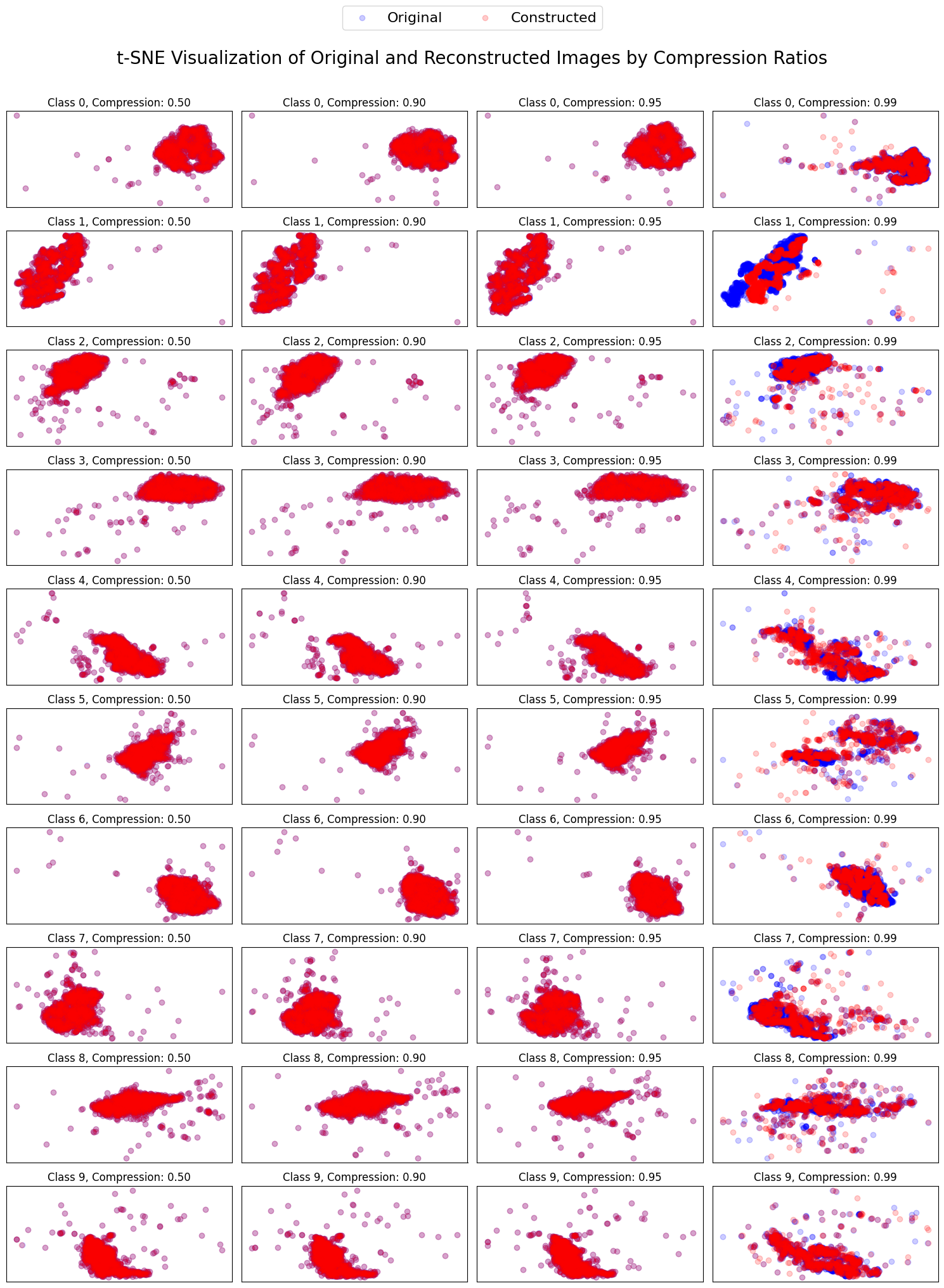
t-SNE (t-distributed Stochastic Neighbor Embedding) is a popular technique for visualizing high-dimensional data in two or three dimensions. It's particularly effective at revealing clusters and patterns in complex datasets. t-SNE works by maintaining the relative distances between points in the original high-dimensional space when projecting them onto a lower-dimensional space. This means that points that are close together in the original data will tend to be close together in the t-SNE visualization, while distant points remain separated. This property makes t-SNE especially useful for exploring the structure of high-dimensional data, such as images or word embeddings, in a more interpretable 2D or 3D format.
In this tutorial, we're using t-SNE to compare the distributions of original images and their autoencoder reconstructions. By plotting both sets of data points on the same t-SNE chart (using different colors, e.g., blue for originals and red for reconstructions), we can visually assess the quality of the reconstruction. If the autoencoder is performing well, the blue and red points should significantly overlap, indicating that the original and reconstructed data have similar distributions. Conversely, if the points are clearly separated, it suggests that the reconstructions differ significantly from the originals, pointing to potential issues with the autoencoder's performance.
One might wonder why t-SNE, which can effectively reduce high-dimensional data to two or three dimensions for visualization, isn't directly used for data compression. There are two major limitations that make t-SNE unsuitable for this purpose:
These limitations highlight why we use purpose-built compression techniques, such as Auto-Encoders, which offer better scalability and can efficiently process new data once trained.
This publication investigated the efficacy of autoencoders as a tool for data compression, with a focus on image data represented by the MNIST dataset. Through systematic experimentation, we explored the impact of varying latent space dimensions on both the compression ratio and the quality of the reconstructed images. The primary findings indicate that autoencoders, leveraging their neural network architecture, can indeed compress data significantly while retaining a considerable amount of original detail, making them superior in certain aspects to traditional compression methods.
