Abstract
Breast cancer is a significant public concern everywhere in the world due to the very high death rates, and as proven by doctors that the earlier the cancer is discovered, the greater the success rate which means lowering the death rates. One of the main tools used to detect breast cancer is the ultrasound images, but the problem is that these ultrasound images contains noises that makes it very hard to read through. There are old filtering techniques that were used to remove these noises such as the average filtering, but in this techniques they were losing very important tiny details in these images that could lead to wrong diagnosing. This research paper shows that by using deep learning techniques, more specifically Convolutional neural network (CNN) Autoencoder, we can remove these noises without losing images details. CNN architecture is designed and trained using four different datasets and a custom dataset that were created using data augmentation techniques, and to measure the performance we used 3 different evaluation metrics PSNR, MSE, and SSIM. There are 40 different training trials were done and in each of these trials the parameters were different. These parameters includes epoch size, batch size, number of filters in each of the CNN layers, and finally the dataset size. The output values shows that deep learning approaches have better results compared to previous papers and previous old filtering techniques.
Methodology
The model that is used is a denoising autoencoder neural network model with a TensorFlow backend and the Keras framework. The purpose of this model is to be able to map noisy input images to clean output images. To accomplish this the input images are first encoded into a lower-dimensional representation which is subsequently decoded to return to the original image space. The input layer is the first of the model’s three main layers. The input layer is the layer where it accepts input data in the format (128,128, 1) where 128x128 denotes a single-channel grayscale image and 128 is the image size. These are the encoder layers that makeup layer 2. Where the encoding is done through convolutional layers. The first layer retains the input’s spatial dimensions by using 128 3x3 filters with ReLU activation and same padding. The feature maps’ spatial dimensions are downsampled by a factor of 2 using the Max pooling layers which have a pool size of 2x2 and the same padding applied. The Max pooling layer comes after each of the three convolutional layers which have 128 filters of 3x3 size and ReLU activation added progressively. The layers of decoders comprise the third main layer. wherein ReLU activation and three convolutional layers with 128 filters of 3x3 size are employed for decoding. Reconstructing the denoised image is the goal of these following layers. The feature maps are upsampled using the upSampling2D layers which have a 2x2 size thereby doubling their spatial dimensions. With a single 3x3 filter and sigmoid activation, the final convolutional layer aims to produce a denoised image.
Block Diagram using Deep Learning (CNN):
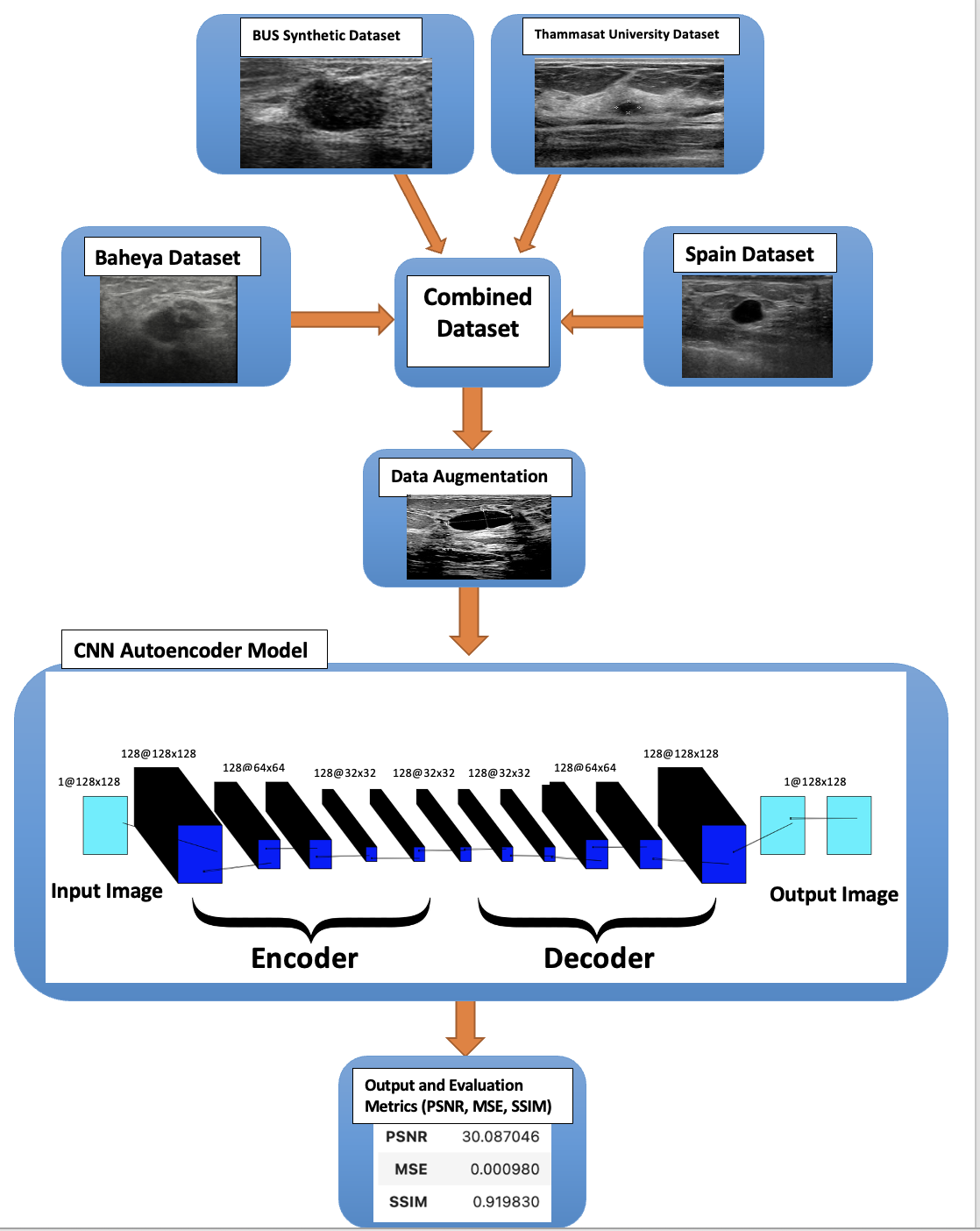
There are 4 different parameters that I changed to achieve the best results. The first main parameter is the epoch’s size, an epoch is the total number of training data iterations in a single cycle to train the CNN model. It is the period during which all training data is used simultaneously. An epoch can also be defined as the number of iterations a training dataset goes through an algorithm. The epoch sizes that were tested are 1, 10, 20, 35, 50, 75, 100, and 300. The second parameter is the batch size, which is the number of samples to go through before changing the internal model parameters. It may be one of the most important actions to ensure that your models operate at their best. The batch sizes that were used were 16 and 64. The third parameter is the number of filters in each layer, and I used 128, and 256 to compare the results. The problem that occurred when doubling the number of filters, is that it takes almost triple the time for each epoch, as shown in the Results chapter. The last parameter that affected the results is the size of the dataset, and this parameter is explained in detail in the ”Dataset” section. There is a total of 40 different trials that were created and compared together to achieve the best results as shown in the ”Results” section.
We measure the CNN Model using three different parameters. The first and most important parameter is the PSNR, which stands for the peak signal-to-noise ratio and the higher it gets the better the outcome. The second parameter is the Mean Square Error (MSE), which is a very important metric for evaluating the performance of predictive models, and our goal is to make it close to 0 as much as possible. The third parameter is the structural similarity index measure (SSIM), and the higher the rate the better the results.
During the evaluation part, we compare the results of the CNN autoencoder with the old filter techniques. The first filtering technique is the Gaussian filter which is a low-pass filter that is used for noise reduction and adds blurring in regions in the image. The main parameter in this type of filtering is the standard deviation parameter. Increasing or a higher standard deviation the more effective in reducing the noise, but it may also lose small details in the image, which is one of the main limitations in previous papers. The second filtering technique is the Median filter, which is a non-linear filter, and it works by replacing each pixel value with the median value within a local neighborhood. It’s very effective in removing salt and pepper noise, it doesn’t lose important details, and it does not blur the image. The third filtering technique that we use to compare our results is the Average filter, and it works by replacing each pixel with the average value of its neighboring pixels. The last filtering technique is the Bilateral filter, which is a non-linear filter. It works by taking the weighted average neighbor pixels, and the weight depends on the distance between the pixel itself and the center pixel. It’s an effective way to remove noise while preserving the edges and small details.
Tools Used
I used Python language and two different notebooks, the first one is Google Colab, which is a hosted Jupyter Notebook service that requires no setup to use and provides free access to computing resources. However, its limitation is that it has a maximum of 12 hours, and to access GPU there is a monthly fee that should be paid. The second notebook is the Kaggle notebook, which is a cloud-computed notebook, where all your code or processes are computed on their cloud servers. Although Kaggle also has a maximum of 12 hours, it has a free GPU that could be used that make the training time three times faster. The computer used is a Macbook Pro M1 Chip, with an 8-core CPU with 4 performance cores and 4 efficiency cores. 8-core GPU, 16-core Neural Engine. The operating system is MacOS.
Datasets Used
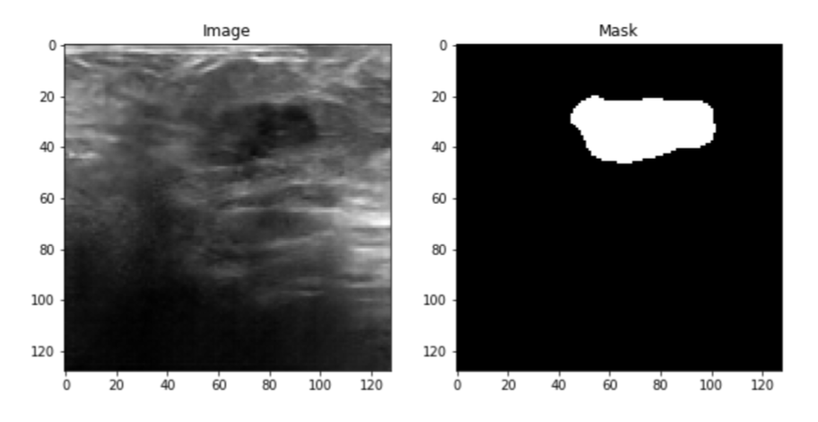
Four datasets were used, the first one is the Baheya dataset which includes a total of 780 ultrasound images. These images are split into three categories Benign, Malignant, and normal, and each category includes 437, 210, and 133 respectively. Also, each ultrasound image has its mask images as shown in the figure below.
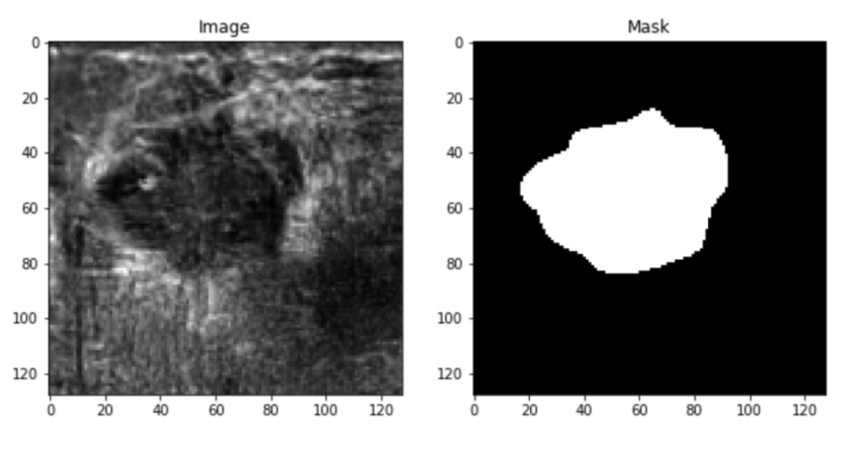
The second dataset is Bus-synthetic-dataset, which consists of 500 breast ultrasound images, and each image has its mask same as the first dataset as shown in the figure below.
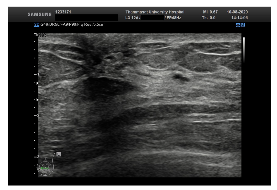
The third dataset is Thammasat University dataset, which consists of 500 breast ultrasound images, however, every image doesn’t have a mask.
The fourth dataset is Spain Dataset sometimes referred to as Dataset B, which consists of 163 images, however, every image doesn’t have a mask.
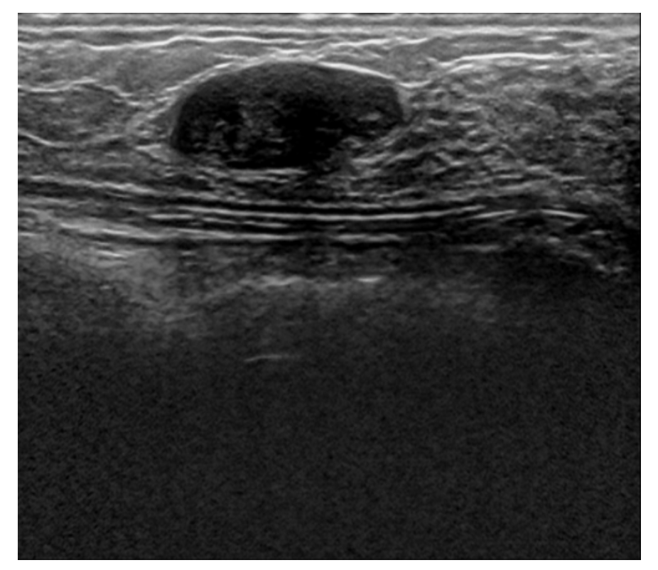
There is training done on the Baheya dataset separately, which means a total of 780 images that are separated into 500 training and 280 testing. Then Combining the Baheya dataset with the Bus-synthetic dataset with a total of 1280 ultrasound images, 900 of them were trained on and the rest 380 for testing. After that Combining the third Thammasat dataset with a total of 1568 images, 1100 images went for training and the rest 468 images for testing. Finally combining all four datasets with a total of 1731 breast ultrasound images, 1200 of them for training and the rest 531 for testing.
Results
Data Augmentation
Data augmentation plays a very important role in improving the accuracy of any CNN model, especially in my project. To improve the model accuracy we need a huge dataset to train the model, however in the medical field it’s very hard to find a large dataset, so one of the solutions is to generate new data from existing data. This could be done easily through any of the machine learning approaches by taking as input the original image and returning the augmented images. However, due to different dark levels in the ultrasound images, this cannot be done because it will lead to the damage of some of the dark images. To solve this problem I created the new data manually by increasing the sharpness and contrast of the images. The data augmentation made the dataset increase from 1731 to 3339.
Results Sorted by PSNR
As shown in the below Table, it’s a summary of all of the 40 trials that were tested on the CNN Autoencoder Model. The first column is the number of trials. The second column is the epochs that range from 1 epoch to 300. The third column is the batch size which is either 16 or 64. The fourth column is the number of filters in each of the CNN auto-encode layers as shown in the ”Model” Section, and each layer it’s either 128 or 256 filters in each layer. The fifth column is the size of the breast ultrasound images, and it’s either the Baheya dataset (780) image, or a combination of the Baheya and Bus-synthetic-dataset, with a total of 1280 images, or 1568 images combining the Thammasat University dataset, or 1731 images combining Spain dataset, and finally it could be 3339 ultrasound images after adding the data augmented dataset. The sixth column is the time taken to train the model, and the column beside it is the average time taken for each epoch. The eighth column is the PSNR, which this table sorted ascendingly according to it. The Last two columns are the rest of the evaluation matrices the MSE, and SSIM.
As mentioned earlier the following table is sorted according to the PSNR, so the last row is the best result I have reached so far. It was 30 epochs, batch size 16, 256 filters in every layer in the model, and a data size of 1568 ultrasound images, which means it combines the Baheya Dataset and Bus-synthetic dataset, as well as the Thammasat Univeristy Dataset. The results as following, PSNR = 30.44, MSE = 0.00090, and SSIM = 0.935 or 93.5%.
| Number Of trials | Epochs | Batch Size | # Of Filters | Dataset Size | Time Taken (min) | Time Taken per epoch (min) | PSNR | MSE | SSIM |
|---|---|---|---|---|---|---|---|---|---|
| 1 | 1 | 64 | 128 | 780 | 2.5 | 2.5 | 15.67 | 0.0270 | 0.365 |
| 2 | 1 | 64 | 256 | 780 | 7.5 | 7.5 | 16.32 | 0.0230 | 0.359 |
| 3 | 1 | 16 | 256 | 780 | 6 | 6 | 16.97 | 0.0200 | 0.364 |
| 4 | 1 | 16 | 128 | 780 | 1.5 | 1.5 | 18.54 | 0.0139 | 0.367 |
| 5 | 1 | 16 | 256 | 1731 | 0.3 | 0.3 | 18.80 | 0.0131 | 0.451 |
| 6 | 1 | 16 | 256 | 1280 | 11.5 | 11.5 | 19.159 | 0.0120 | 0.588 |
| 7 | 1 | 16 | 256 | 3339 | 0.5 | 0.5 | 20.59 | 0.0087 | 0.564 |
| 8 | 10 | 64 | 128 | 780 | 15 | 1.5 | 21.56 | 0.0069 | 0.594 |
| 9 | 10 | 64 | 256 | 780 | 50 | 5 | 22.22 | 0.0059 | 0.657 |
| 10 | 20 | 64 | 128 | 780 | 30 | 1.5 | 22.38 | 0.0052 | 0.677 |
| 11 | 50 | 64 | 128 | 780 | 65 | 1.3 | 23.65 | 0.0043 | 0.757 |
| 12 | 50 | 64 | 256 | 780 | 252 | 5.04 | 23.79 | 0.0041 | 0.783 |
| 13 | 10 | 16 | 128 | 780 | 13 | 1.3 | 24.03 | 0.0039 | 0.793 |
| 14 | 50 | 16 | 256 | 3339 | 9.5 | 0.18 | 24.15 | 0.0038 | 0.892 |
| 15 | 10 | 16 | 256 | 1731 | 1 | 0.1 | 24.20 | 0.0037 | 0.822 |
| 16 | 1 | 16 | 256 | 1568 | 14.5 | 14.5 | 24.23 | 0.0037 | 0.728 |
| 17 | 10 | 16 | 256 | 780 | 50 | 5 | 24.28 | 0.0037 | 0.780 |
| 18 | 10 | 16 | 256 | 1280 | 88 | 8.8 | 24.480 | 0.0035 | 0.800 |
| 19 | 10 | 16 | 256 | 3339 | 2 | 0.2 | 24.69 | 0.0033 | 0.813 |
| 20 | 300 | 64 | 128 | 780 | 356 | 1.18 | 24.85 | 0.0032 | 0.824 |
| 21 | 20 | 16 | 256 | 3339 | 3.6 | 0.19 | 25.02 | 0.0030 | 0.838 |
| 22 | 20 | 16 | 128 | 780 | 42 | 1.18 | 25.17 | 0.0030 | 0.844 |
| 23 | 100 | 64 | 128 | 780 | 356 | 1.18 | 25.38 | 0.0028 | 0.828 |
| 24 | 20 | 16 | 256 | 780 | 98 | 4.9 | 25.42 | 0.0028 | 0.831 |
| 25 | 20 | 16 | 256 | 1731 | 2 | 0.1 | 25.70 | 0.0026 | 0.884 |
| 26 | 20 | 16 | 256 | 1280 | 175 | 8.75 | 25.857 | 0.0025 | 0.857 |
| 27 | 20 | 64 | 256 | 780 | 100 | 5 | 25.92 | 0.0025 | 0.850 |
| 28 | 100 | 16 | 128 | 780 | 117 | 1.17 | 26.35 | 0.0023 | 0.881 |
| 29 | 35 | 16 | 256 | 1568 | 367 | 10.48 | 26.63 | 0.00217 | 0.875 |
| 30 | 50 | 16 | 128 | 780 | 58 | 1.16 | 26.81 | 0.0020 | 0.896 |
| 31 | 35 | 16 | 256 | 1280 | 295 | 8.43 | 26.826 | 0.0020 | 0.885 |
| 32 | 50 | 16 | 256 | 780 | 267 | 5.34 | 27.22 | 0.0018 | 0.904 |
| 33 | 100 | 16 | 256 | 1731 | 8.8 | 0.088 | 27.815 | 0.0016 | 0.916 |
| 34 | 50 | 16 | 256 | 1731 | 4.5 | 0.09 | 28.00 | 0.0015 | 0.921 |
| 35 | 10 | 16 | 256 | 1568 | 109 | 10.9 | 28.42 | 0.0014 | 0.88 |
| 36 | 60 | 16 | 256 | 1568 | 620 | 10.33 | 28.73 | 0.00134 | 0.912 |
| 37 | 20 | 16 | 256 | 1568 | 208 | 10.4 | 28.81 | 0.0013 | 0.906 |
| 38 | 50 | 16 | 256 | 1280 | 431 | 8.62 | 30.037 | 0.0009 | 0.927 |
| 39 | 75 | 16 | 256 | 1280 | 593 | 7.91 | 30.087 | 0.00098 | 0.919 |
| 40 | 30 | 16 | 256 | 1568 | 310 | 10.33 | 30.44 | 0.00090 | 0.935 |
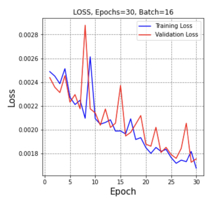
The PSNR were increasing proportionally to the number of epochs until it reached 30 epochs then it started to decrease. This means it reached its maximum at 30 because after that the model started to memorize the data, in other words, it’s a sign of overfitting. Rather than learning to generalize from the training data overfitting happens when a model becomes too adept at memorization of the data noise. This means that the model does well on training data but badly on test or validation data that has not been seen. To overcome this problem there is more than a solution, we could stop earlier as done in this experiment. Also, we could increase the data size by applying transformations like rotation, flipping, or scaling can help the model generalize better. Another solution is to decrease the number of filers or layers in the model if it’s too complex.
We can conclude from the following table that PSNR values increase proportionally with the number of filters. Increasing the number of filters to more than 256 will lead to both advantages and disadvantages. First of all, it will lead to better performance because the data will go through more filters; however, it will increase the computational cost of both training and validation. The model needs more memory and processing power for both forward and backward passes during training when there are more filters added to it. As well as, there is a risk of over-fitting which happens when increasing the epoch size as mentioned earlier. Finally, it requires more than double the training time, which is a limitation mentioned earlier in the ”tools used” section.
We can conclude from the following data that even though 1731 images should have had a higher PSNR, but they didn’t. This is because the Spain dataset has different gray levels and contrast levels than the rest of the datasets, which means when the model started to train with datasets that are not similar to each other it started to decrease in performance, which led to lower PSNR results.
Also, we can see the same problem when adding the custom dataset which consists of 3339 breast ultrasound images, because this dataset was too dark due to the high contrast added to it, which caused a loss of important details in the ultrasound at the same time it’s different that Baheya, Bus synthetic, and Thammasat University datasets.
Results Analysis
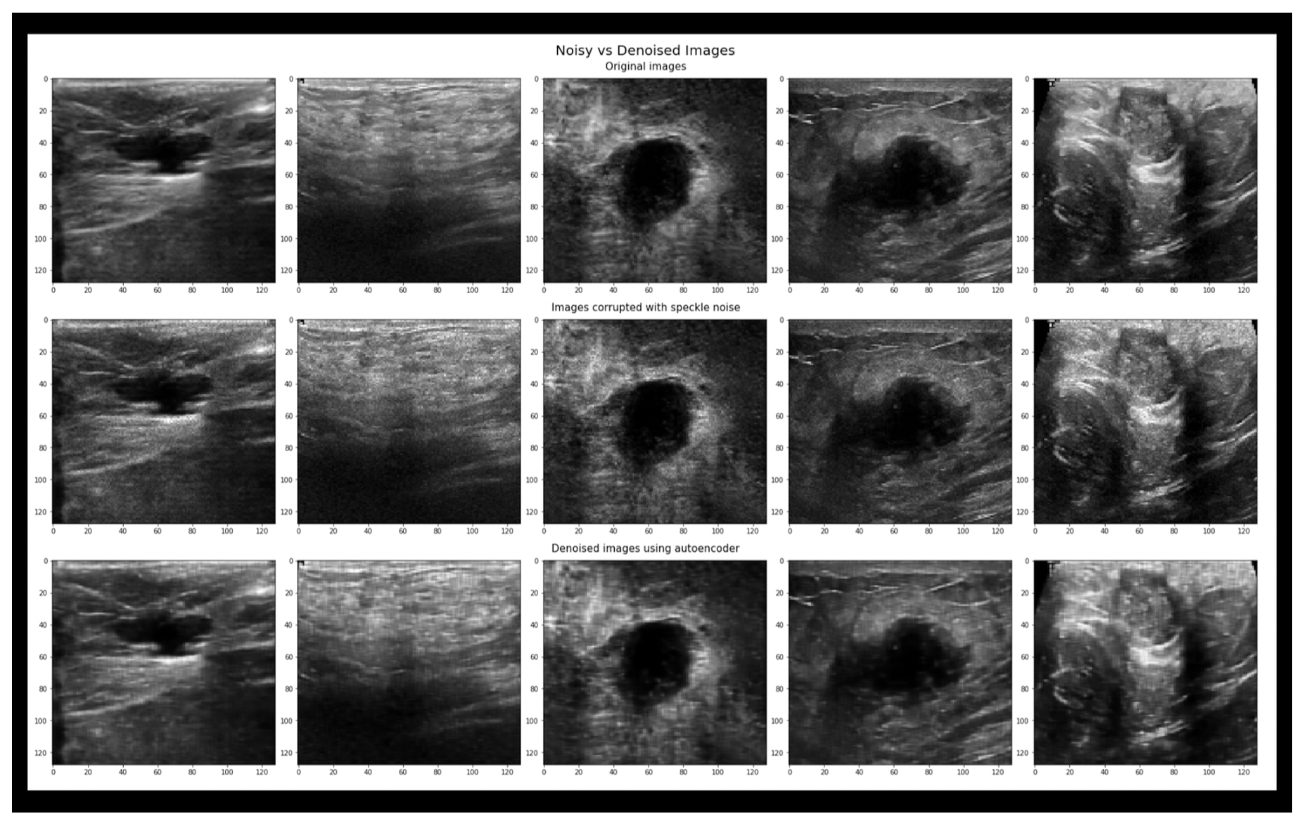
The best PSNR results we have reached so far, as mentioned earlier is (PSNR = 30.44), while at the Median filter, it was (PSNR = 25.362), Gaussian filter (PSNR = 27.541), Average filter (PSNR = 24.934), and Bilateral Filter (PSNR = 23.675), as shown in details at table II, and we can conclude from these results that the CNN Autoencoder is better that the other filtering techniques by 20.02%, 10.52%, 22.08%, and 28.57%, respectively. These results came at an epoch size of 30, batch size of 16, and 256 filters in each of the CNN Layers using the combined dataset which consists of 1568 breast ultrasound images. Below is the training vs validation loss graph , as well as the output image compared to old filtering techniques.
While the best MSE results we have reached so far, is (MSE = 0.0009), while at the Median filter, it was (MSE = 0.0022), Gaussian filter (MSE = 0.0017), Average filter (MSE = 0.0028), and Bilateral Filter (MSE = 0.0034) and we can conclude from these results that the CNN Autoencoder is better than the other filtering techniques. These results came at an epoch size of 50, batch size of 16, and 256 filters in each of the CNN Layers using the combined dataset which consists of 1280 breast ultrasound images, also the same MSE came at an epoch size of 30, batch size 16, and 256 filters in each of the CNN Layers, and a dataset of size 1568 ultrasound images.
The best SSIM results we have reached so far is (SSIM = 93.5%) while at Median filter it was (SSIM = 78.5%), Gaussian filter (SSIM = 87.1%), Average filter (SSIM = 76.9%), and Bilateral Filter (SSIM = 70.7%) and we can conclude from these results that the CNN Autoencoder is better than the other filtering techniques. These results came at an epoch size of 30, batch size of 16, and 256 filters in each of the CNN Layers using the combined dataset which consists of 1568 breast ultrasound images.

Comparing results with existing work
Comparing my work with previous work, I was able to overcome some of the limitations. In the CNN autoencoder model, it can work with different noise levels, not a specific noise level. This means the same model could work with any dataset; however, if there are two datasets and each of them has a different noise level or different contrast levels, it can’t be combined because as shown in the ”result” section, that when combining the data augmented dataset it resulted in a lower PSNR value.
As shown in one of the papers that using Dilated Convolution Autoencoder Denoising Network it resulted in PSNR 29.96 at 0.7 dB and SSIM: 93.13%, while my model resulted in PSNR 30.44 and SSIM at 93.5%, which shows the add on value my model adds. However, the Dilated Convolution Autoencoder used by the referenced paper trained the same model with a lower standard deviation, and this time they had a higher PSNR and SSIM of 34.32 and 97.87%.
As well as comparing to existing work that they used ten different techniques Lee Filter, Frost Filter, Shock Filter, Bilateral Filter, AD, SRAD, DWT, MBF, Thresholding Technique and the Anisotropic Diffusion Method, their proposed method, and the highest PSNR they reached is 30 and SSIM 90.3%, which shows that my autoencoder model has a higher PSNR and SSIM values.
Compared to my key reference paper, they used five different techniques to remove the noise, Frost, Kaun, Visu, Bayes, and their proposed new method, and at the variance of 0.06, the highest PSNR they reach is 29.837, which still lower to my highest PSNR values; however, when decreasing the variance to 0.02, it reached to a PSNR value of 32.614.
Another limitation that was fixed is not losing tiny details, because as shown in the resulting image all details are still shown; however, using old filtering techniques will lead to loss of data due to lowering image resolution. Also, a problem that some of the papers faced was that they used a low-processor computer which limited their training, but using Kaggle GPU it was able to solve this issue and reach an epoch size of 300.
Conclusion
In this paper, we discussed the importance of ultrasound images in medical fields, especially in breast cancer detection, where early detection results in better diagnosis. The problem we are aiming to solve is that in these images there are noises that make important diagnostic features not clear to doctors or to AI models that detect if there is cancer. To solve this problem our aim is to create a Generative-AI Model for Noise Detection in Breast Cancer Ultrasound images, to remove these noises without losing important details.
We started by discussing different old techniques, such as average filtering and median filtering, that were used to detect and filter the noises from breast ultrasound images. The disad- vantage of these techniques is that they lose small details that could lead to removing very important details and resulting in a wrong diagnosis. To solve this problem we used deep learning techniques, specifically CNN Auto-encoder. This is done through a two-step process, the first one is encoding the input images into a lower-dimensional representation and then decoding them to reconstruct the original image. To achieve the best results we have changed some of the parameters and compared the output. The parameters are the epoch size, batch size, and number of filters in each layer in the Autoencoder, as well as changing the dataset size by combining 4 different datasets and building my custom data using data augmentation reaching a total of 3339 ultrasound images. We compared the results using 3 main evaluation metrics PSNR, MSE, and SSIM. The best PSNR we have reached is 30.44, which is a high value compared to previous papers.
Future Work
Although we were able to achieve very good results com- pared to previous papers, there is more work that could be done to achieve higher PSNR values. First of all, is to explore alternative approaches, such as the CNN UNet Model, and compare the outcome with the CNN Autoencoder Model. Sec- ondly, one of the main limitations is that there is a minimum number of ultrasound images dataset, so increasing the dataset could lead to better results. This could be done using Data Augmentation. Finally, approve that the outcome images are useful to the doctors and medical fields by approving it from the approved companies, and this could be done by creating a survey.