Abstract

This project is focusing on developing an advanced electricity consumption forecasting model
using machine learning techniques to enhance the versatility and accuracy of the forecasts.
Using traditional statistical models may result in failing to capture the non-linear nature of
modern energy system, particularly when they are influenced by weather, global crises such
as COVID-19 and economic changes.
This project is being developed to cap this gap by integrating different machine learning
models such as TBATS, ARIMA and SARIMA to analyse huge datasets and reveal hidden
patterns in different power consumption zones of Morocco.
The approach is delivering high scalability and adaptability, so it can be used on different
economic, climatic and geographical conditions. It also ensures reliability among all datasets
by using some special techniques for augmenting the data (synthetic data generation) and
feature engineering. This methodology includes data collection, data pre-processing, model
selection and evaluation then final deployment using web interface.
ARIMA, TBATS and SARIMA are the major machine learning models used, all of these are
evaluated for their performance. In this project, they will contribute to more efficient energy
production and more sustainable energy management practices.

Methodology

The procedure for electrical energy consumption prediction using machine learning follows a
methodical approach that have steps such as data collection, model selection, pre-processing,
training, evaluation and model deployment. The aim is to implement a highly adaptive and
accurate predictive model that can handle sudden consumption shifts, non-linear trends and
some external factors such as economic changes and climate fluctuations.
2.1. DATA COLLECTION AND PREPROCESSING
Step one is gathering historical data from various sources like energy suppliers, weather
forecasts, smart meters and government databases etc. These datasets have information
related to energy consumption, external factors affecting energy demand and economic
indicators and weather conditions. In real world, data is usually incomplete or with full of
inconsistencies like null values, duplicate values etc, so it requires preprocessing techniques
such as Exploratory Data Analysis which in end helps to remove duplicates, handling missing
values and smoothening of noise to ensure high data veracity.
Synthetic Data Generation:
For robustness of model and improved accuracy of the forecasts synthetic data is generated
by adding noise around the standard deviation. It will help to simulate the changes in energy
consumption and will help to reduce overfitting especially when training is being done on a
limited dataset.
2.1.1 FEATURE SELECTION AND ENGINEERING
Refining input variables to improve model performance can be done by feature selection and
engineering. This project is highlighting transforming the data distribution after handling
outliers to get a Gaussian distribution, instead of using highly mathematical techniques like
Recursive Feature Elimination and Principal Component Analysis.
Managing Outliers and Data Distribution :
• Statistical methods like Inter Quartile Range(IQR) visualized through box plots and Z
score analysis are helpful in outlier detection. Box-cox and Yeo-Johnson transformation are used to normalize skewed distributions,
both of these are part of data transformation techniques used in this project.
• Extreme values should be handled with caution as they are responsible for data
sensitivity, so to make data less sensitive Robust Scaling is used. This scaling is used
before Standard scaling for uniform distribution of data across all the features.
The steps mentioned above helps to improve the stability of the machine learning models and
makes them more resistant to changes in energy consumption trends.
2.2 MODEL SELECTION
Selecting the right forecasting model is crucial to forecast electrical energy consumption with
high accuracy. Considering the complex and dynamic nature of energy demand patterns, this
project uses a combination of time series models (ARIMA, SARIMA, TBATS) suited for different
aspects of forecasting.

1. Autoregressive Integrated Moving Average (ARIMA):
   • ARIMA proves effective at finding linear relationships between time series data points
   because of its wide use as a statistical model. The data collection works effectively for
   short-term power predictions in situations with predictable patterns. Due to its
   straightforward nature this model functions as a dependable tool which makes it easily
   understandable.
   • The main drawback of using ARIMA occurs when researchers need to analyse unsteady
   data because the model fails to process data affected by seasonal changes and
   weather patterns. The technique does not provide immediate responses to either
   sudden demand changes or lengthy interdependent relationships.
   • ARIMA represents the fundamental approach to model comparison because it helps
   establish advanced prediction methods to handle short-term pattern fluctuations in
   energy usage.
2. Seasonal ARIMA(SARIMA):
   • ARIMA forecasts become more effective through SARIMA because it includes seasonal
   pattern analysis which suits energy use prediction of cyclical data patterns. The
   method enhances forecasting precision in datasets that display repetitive pattern consumption over daily or weekly or annual cycles but it keeps the interpretability
   features of ARIMA.
   • Adjusted use of SARIMA models with several seasonal components might lead to
   increased computational complexity. It proves less effective than alternative methods
   for dealing with unexpected changes which do not follow established seasonal
   patterns.
   • The modelling of repeated seasonal trends in SARIMA produces better results than
   ARIMA since it provides precise estimates for electricity use.
3. Trigonometric Functions, Box-Cox Transformation, ARMA Error, Trend and Seasonal
   Components(TBATS)
   • This model is specifically designed for handling multiple non-linear trends and
   seasonality. It is best suitable for estimating energy usage and long-term patterns.
   Variations occurred by factors like climate changes and economical changes are
   managed by TBATS.
   • TBATS requires a lot of computing power and has longer training times, especially for
   large datasets. Its hyperparameters must also be changed for performance to be
   optimized.
   • Computing power is much needed by TBATS and it has longer training time for large
   datasets. Hyperparameters must also be varied for performance optimization.
   Seasonal energy usage is affected by daily peaks and weekly demand cycles, this model
   is important for collecting these issues and helps to enhance prediction accurately.
   By using these three models, our project provides a complete comparative analysis by
   selecting the best approach for precise energy consumption projections.
   2.3 MODEL CREATION
   After selecting model, next stage is achieving unbiased evaluation for this it is necessary to
   split the pre-processed dataset into training and test sets. To improve the robustness of the
   model, this energy consumption dataset is transformed using synthetic data generation. For
   the augmentation of data, noise around standard deviation is used.
   Data Scaling and Transformation
   Outlier detection and data distribution transformation are applied to improve the model
   performance. The data is transformed into a Gaussian distribution using the following
   methods:
   • Robust Scaling : reduces the impact of outliers.
   • Power Transformation (Yeo-Johnson and Box-Cox): stabilizes the variance and
   normalizes skewed data.
   • Default scaling: Ensures that the data is evenly distributed before the model is trained.
   Hyperparameter Tuning
   Models are fine-tuned using techniques like auto-ARIMA to optimize parameters such as p, d,
   q (ARIMA/SARIMA) and seasonal components (SARIMA/TBATS).
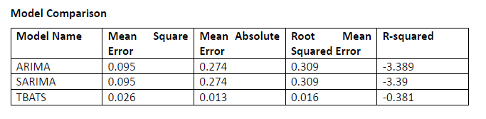
   Evaluation metrics include:
   • Mean Absolute Error (MAE)
   • Mean Square Error(MSE)
   • Root Mean Squared Error (RMSE)
   • R² Score
   This structured model training approach guarantees a fair comparison between different
   forecasting techniques.
   2.3.1 TRAIN AND TEST SPLIT
   The dataset is then split into training and test data to make sure that the model generalizes
   very well to new, unknown data. This makes the ratio between the train/test split as follows:
   80:20%. This implies that 80% of the historic energy consumption dataset is used in training
   and the remaining 20% for the validation and the test phase, respectively.
   Time Series Allocation :
   The consumption of energy is time dependent. Thus, simple random allocation is avoided.
   Instead, the dataset is split into a time series where older data is used for training and newer
   data is used for testing. This allows the model to learn past trends and apply them to predict
   the future.
   2.3.2 MODEL EVALUATION
   After training, the models are rigorously evaluated using multiple metrics to assess accuracy,
   robustness, and predictive power. The following key evaluation metrics are considered:
4. MAE, or mean absolute error :
   It calculates the mean absolute difference (MAE) between the actual and predicted energy
   consumption figures. It provides a straightforward metric of prediction accuracy by ignoring
   the direction of the errors. Since it makes fewer predictions, a model with a lower MAE value
   is more accurate.
5. Root mean squared error, or RMSE :
   RMSE surpasses MAE because it penalizes larger deviations more harshly. Because RMSE
   squares the errors before averaging them, it magnifies the impact of significant errors and is
   hence particularly helpful for detecting sharp variations in energy usage. A model is more
   predictive and less likely to make large forecasting errors if its RMSE is smaller.
6. The R2 score error:
   This is often known as the coefficient of determination evaluates how well a model takes
   dataset volatility into account. It determines the proportion of variability in real energy use
   that the prediction model can explain. The model is highly dependable in forecasting when its
   R2 value is close to 1, successfully accounting for most changes.
7. Analysing Model Performance :
   Each forecasting model has unique benefits and drawbacks that influence how well it matches
   different patterns in energy consumption:
   • For short-term forecasting, the Auto-Regressive Integrated Moving Average, or ARIMA,
   is a useful tool since it effectively captures linear trends. It struggles with intricate
   seasonal correlations and long-term fluctuations, though.
   • By adding seasonal patterns, SARIMA (Seasonal ARIMA), an extension of ARIMA,
   improves forecasting accuracy and is better suited for datasets where consumption is
   greatly influenced by periodic shifts.
   • Considering that it effectively manages numerous seasonal patterns, non-linearity, and
   unpredictable variations in energy demand, the TBATS model is anticipated to produce
   the most accurate projections.
   The most accurate and trustworthy forecasting technique is found for practical application by
   examining these performance indicators and model behaviours, guaranteeing better energy
   management and planning.
   2.4. DEPLOYMENT
   The real-time forecasting system receives the best models from model evaluation and training
   procedures subsequent to model deployment. The deployment process includes:
   • Streamlit UI integration: Streamlit is capable of fetching real-time changes in data as
   it directly fetching data from the python code and any changes that occurs in data or
   code are reflected in real-time .By using Streamlit we can provide a highly interactive
   and user friendly Web App .
   • Automatic model updates: The forecasting models get trained intermittently using
   latest consumption data to adapt to evolving energy pattern changes.
   • Scalability and Adaptability: The forecasting system adopts scalable design principles
   which permit easy adaptation into smart grid and energy management platforms.
   The adopted methodology enables the project to develop a forecasting system with high
   accuracy that enables adaptation and efficiency to benefit energy optimization initiatives and
   sustainability goals.

Results

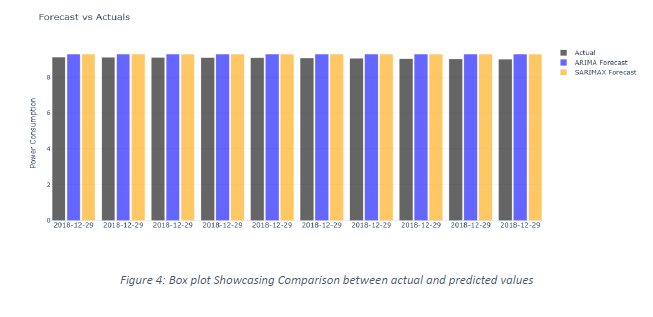
The research evaluated three time series forecasting approaches including ARIMA, SARIMA
and TBATS to forecast future patterns. The ARIMA model demonstrated solid results when
analysing stationary data although it works best when working with data that lacks substantial
seasonality and trends. The model produced forecasts that were less accurate because of its
difficulty in dealing with datasets that presented strong seasonal patterns.
The SARIMA analysis achieved superior results than ARIMA when dealing with seasonal time
series. SARIMA achieved better forecasting accuracy because it integrated seasonal variance
to detect underlying seasonal patterns. ARIMA failed to produce satisfactory results within
patterns exhibiting monthly or quarterly seasonality until the dataset demonstrated these
periodic features.
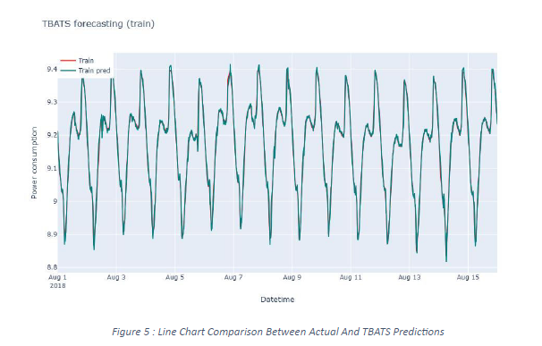
The TBATS model generated the superior results among these time series models because it
handles multiple seasonal cycles and incorporates nonlinear trends on complex seasonality
data. The TBATS model efficiently handled multiple seasonal periods by allowing complex
seasonal effects modelling and produced better forecasts than both ARIMA and SARIMA
during time-dependent seasonality changes.
TBATS produced the minimum RMSE from all models tested followed by SARIMA while ARIMA
had the maximum error values. The analysis indicates that TBATS demonstrates the best
capability to analyse intricate time series datasets.
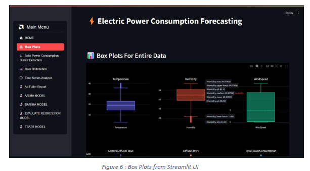
UI deployment
For UI deployment we have used Streamlit which allows the development of creative, dynamic
and real-time data driven apps using external data. It has been designed to display the
forecasting results of electric power consumption using various time series models.
This web application sets up a page with a sidebar menu that helps with navigation through
different sections of visualizations like Boxplots , Data Distributions and time series models
like ARIMA , SARIMA and TBATS.
Boxplots are used to visualize the distribution of different features in the dataset with
and without scaling and skewness.
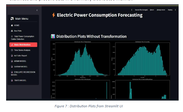
The Data Distribution Plots for various features are used for showing that
transformation using boxcox and power transformer (yeo-johnson) can reduce
skewness and present data in a normally distributed manner.
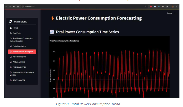
The Time Series Analysis plot gives the total power consumption over time and analyse
the autocorrelation to understand patterns and seasonality.
The Stationary Tests are performed using ADF and KPSS tests to check if time series
data is stationary for the purpose of accurate forecasting.
Forecasting Models :
Models like ARIMA , SARIMA and TBATS are used for making predictions and evaluating
performance metrics like MSE , MAE , RMSE and R-squared.
The Web application has used Plotly library for creating interactive and visually appealing plots
that are user friendly and provides summary of model performance.
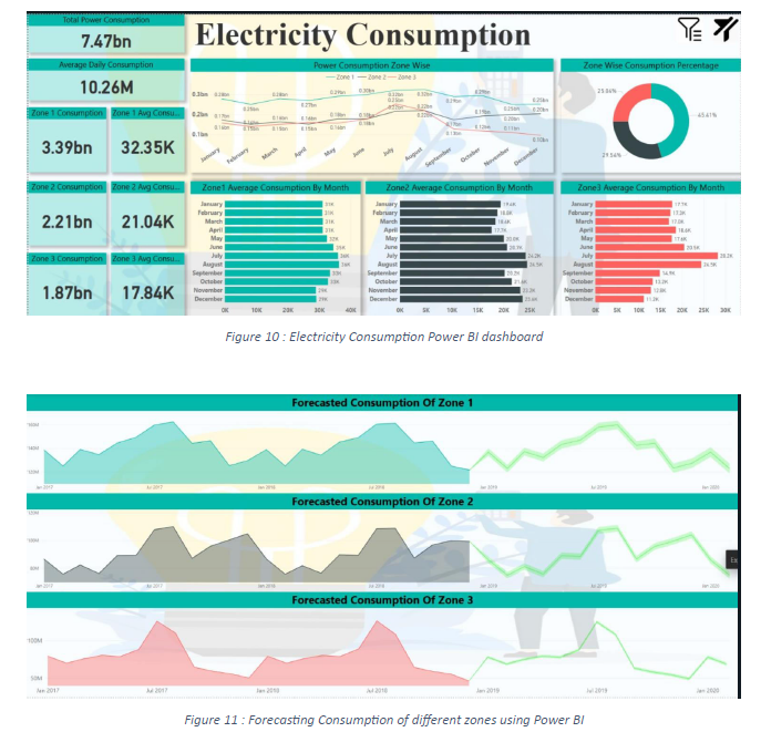
Power BI Dashboard
Power BI dashboard represents zone wise power consumption trend with interactive filters
and visuals, also we have used seasonal forecasting of next sixteen months using line charts.