Abstract

Traditional investment strategies often struggle to respond quickly to market volatility. Investors need models that not only forecast market trends but also adjust asset allocation to maximize returns and control risk. This project explores how we can apply machine learning and deep learning techniques to forecast future prices and use those forecasts to make better portfolio decisions.

Methodology

📊 Task 1: Data Preprocessing and EDA

• Extracted 10-year historical data using YFinance

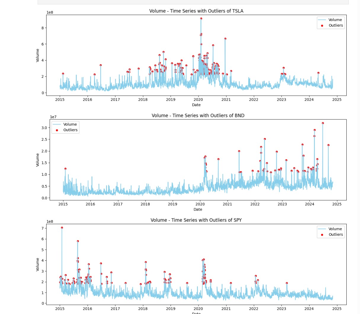
• Cleaned and normalized price, volume, and volatility data

• Visualized price trends, volatility, and return anomalies

• Decomposed seasonal/trend/residual patterns

        """
        Fetches historical data for each symbol and saves it as a CSV.

        Returns:
        - dict: Dictionary with symbol names as keys and file paths of saved CSV files as values.
        """
        data_paths = {}
        
        for symbol in symbols:
            try:
                print(f"Fetching data for {symbol} from {start_date} to {end_date}...")
                data = pn.data.get(symbol, start=start_date, end=end_date)
                # Save to CSV
                file_path = os.path.join(self.data_dir, f"{symbol}.csv")
                data.to_csv(file_path)
                data_paths[symbol] = file_path
                print(f"Data for {symbol} saved to '{file_path}'.")

            except ValueError as ve:
                error_message = f"Data format issue for {symbol}: {ve}"
                if self.logger:
                    self.logger.error(error_message)
                else:
                    print(error_message)

            except Exception as e:
                error_message = f"Failed to fetch data for {symbol}: {e}"
                if self.logger:
                    self.logger.error(error_message)
                else:
                    print(error_message)

        return data_paths

🔮 Task 2: Forecasting Models

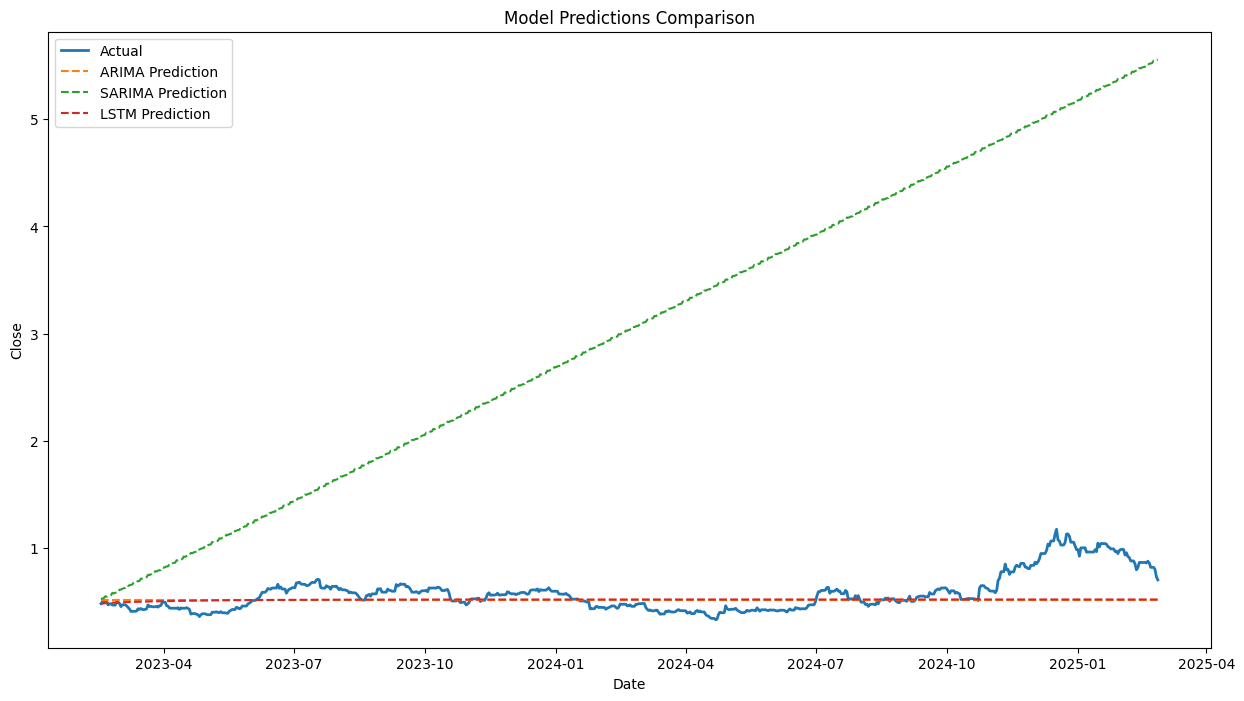
• Built classical (ARIMA/SARIMA) and neural (LSTM) models

• Trained/tested models using walk-forward validation

• Optimized parameters (e.g., auto_arima)

• Evaluated using MAE, RMSE, MAPE

def train_arima(self):
        """Train ARIMA model using auto_arima."""
        try:
            # Check if train and column are valid
            if self.train is None or self.column not in self.train.columns:
                raise ValueError(f"Invalid data: 'train' is None or '{self.column}' column is missing.")
            
            self.logger.info("Training ARIMA model")
            model = pm.auto_arima(self.train[self.column], seasonal=False, trace=True, error_action='ignore',
                                suppress_warnings=True, stepwise=True)
            self.model['ARIMA'] = model
            print(model.summary())
            self.logger.info(f"ARIMA model trained with parameters: {model.get_params()}")
        except Exception as e:
            self.logger.error(f"Error in ARIMA training: {e}")
            raise ValueError("ARIMA model training failed") from e

    def train_sarima(self, seasonal_period=5):
        """Train SARIMA model using auto_arima."""
        try:
            # Check if train and column are valid
            if self.train is None or self.column not in self.train.columns:
                raise ValueError(f"Invalid data: 'train' is None or '{self.column}' column is missing.")
            
            self.logger.info("Training SARIMA model")
            model = pm.auto_arima(self.train[self.column], seasonal=True, m=seasonal_period,
                                start_p=0, start_q=0, max_p=3, max_q=3, d=1, D=1,
                                trace=True, error_action='ignore', suppress_warnings=True)
            self.model['SARIMA'] = model
            print(model.summary())
            self.logger.info(f"SARIMA model trained with parameters: {model.get_params()}")
        except Exception as e:
            self.logger.error(f"Error in SARIMA training: {e}")
            raise ValueError("SARIMA model training failed") from e

📅 Task 3: Market Trend Forecasting

• Forecasted 6–12 month stock prices

• Interpreted confidence intervals and expected volatility

• Identified opportunities and risks in asset behavior

💰 Task 4: Portfolio Optimization

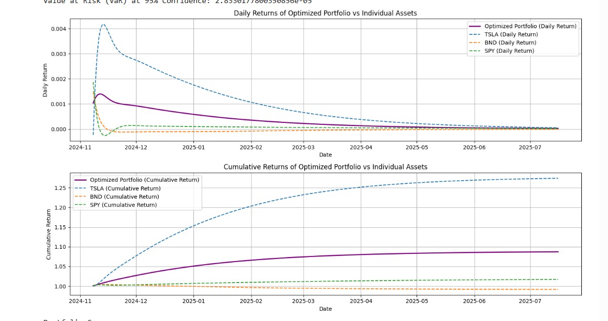
• Used predicted prices for TSLA, SPY, BND

• Computed expected returns, covariance matrix

• Applied Sharpe Ratio-based optimization

• Simulated performance with cumulative return plots and volatility analysis

def optimize_portfolio(self):
        """
        Optimize portfolio weights to maximize the Sharpe Ratio.

        Returns:
        - Dictionary with optimal weights, expected return, risk, and Sharpe Ratio.
        """
        def neg_sharpe_ratio(weights):
            return -self.portfolio_statistics(weights)[2]
        
        constraints = ({'type': 'eq', 'fun': lambda x: np.sum(x) - 1})
        bounds = tuple((0, 1) for _ in range(len(self.df.columns)))
        initial_weights = self.weights

        optimized = minimize(neg_sharpe_ratio, initial_weights, bounds=bounds, constraints=constraints)
        if not optimized.success:
            self.logger.warning("Optimization may not have converged.")
        
        optimal_weights = optimized.x
        optimal_return, optimal_risk, optimal_sharpe = self.portfolio_statistics(optimal_weights)
        self.logger.info("Optimized portfolio - Weights: %s, Return: %.4f, Risk: %.4f, Sharpe Ratio: %.4f",
                         optimal_weights, optimal_return, optimal_risk, optimal_sharpe)
        
        return {
            "weights": optimal_weights,
            "return": optimal_return,
            "risk": optimal_risk,
            "sharpe_ratio": optimal_sharpe
        }

    def risk_metrics(self, confidence_level=0.95):
        """
        Calculate key risk metrics, including volatility and Value at Risk (VaR).

        Parameters:
        - confidence_level: Confidence level for VaR calculation (default is 95%).

        Returns:
        - Dictionary containing 'volatility' and 'VaR_95' (Value at Risk at 95% confidence).
        """
        daily_returns = self.df.pct_change().dropna()
        portfolio_daily_returns = daily_returns.dot(self.weights)
        
        volatility = portfolio_daily_returns.std() * np.sqrt(252)
        var_95 = np.percentile(portfolio_daily_returns, (1 - confidence_level) * 100)
        
        self.logger.info("Portfolio Volatility: %.4f, Value at Risk (VaR) at 95%%: %.4f", volatility, var_95)
        return {"volatility": volatility, "VaR_95": var_95}

Results