Introduction

1.1 Background
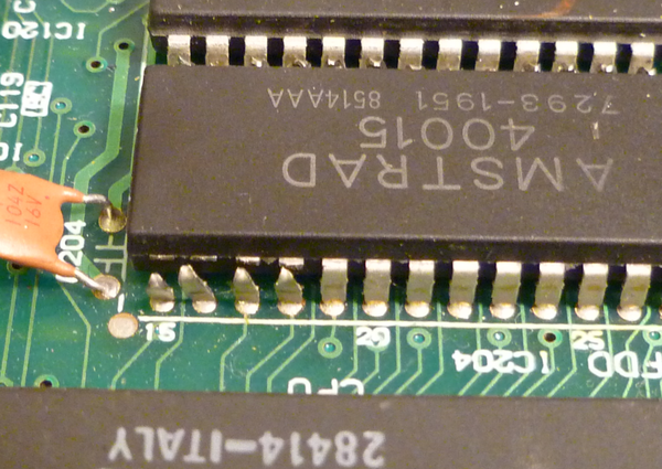
Integrated Circuits (ICs) are the backbone of modern electronics, serving as the critical components that enable complex computations in devices ranging from mobile phones to medical instruments. The leads or pins of ICs are responsible for connecting the internal circuitry to the external world. These leads, typically made from metal, often undergo various mechanical and thermal stresses during the manufacturing process, making them susceptible to defects that can undermine the performance and reliability of the entire IC.

Defect detection in IC leads is vital to the production process. Traditional manual inspection methods are not only time-consuming but also prone to human error, especially when the inspection must be performed under strict quality control conditions. In recent years, automated systems utilizing advanced image processing and machine learning algorithms have been developed to improve the accuracy, efficiency, and scalability of defect detection systems.

1.2 Problem Statement
Despite significant advancements in automated defect detection, current systems still face several challenges, including low detection rates for subtle defects, such as micro-cracks or uneven soldering. Additionally, traditional systems often suffer from high false positive rates, which results in unnecessary rejections of good ICs, thus increasing costs. The variability of defect types further complicates detection tasks, as some defects may appear in a wide variety of forms, making them harder to recognize using conventional computer vision techniques.

1.3 Objective of the Study
The objective of this study is to develop a deep learning model capable of accurately detecting various types of defects in IC leads by leveraging high-resolution images captured during the manufacturing process. This study investigates the use of Convolutional Neural Networks (CNNs), specifically the pre-trained VGG16 architecture, to improve the detection accuracy by fine-tuning the model to the task of IC lead defect detection. By doing so, this research aims to:

• Enhance the accuracy of defect detection through the use of state-of-the-art machine learning techniques.
• Address challenges such as data imbalance and overfitting through advanced data augmentation techniques.
• Provide a reliable automated solution for real-time defect detection that can be integrated into existing manufacturing lines.

1.4 Scope of the Study
This study focuses on detecting common defects in IC leads, including but not limited to, non-uniform color, tooling marks, exposed copper, bent or nonplanar leads, and excess solder. The methodology developed is primarily applicable to the electronics manufacturing industry and aims to support the development of quality assurance systems that can operate autonomously, reducing the need for human intervention and improving overall production efficiency.

Related work

2.1 Traditional Defect Detection Approaches
In the past, defect detection in IC leads was largely handled through traditional image processing techniques, such as edge detection, thresholding, and template matching. These methods rely heavily on manually defined rules and heuristics to identify defects, making them highly sensitive to variations in lighting conditions, IC orientations, and surface textures. While effective in some cases, these approaches have limitations in handling complex or previously unseen defect types, leading to false positives and missed defects.

2.2 Machine Learning in Defect Detection
In recent years, machine learning (ML) approaches have emerged as a powerful tool for improving defect detection. ML models, particularly supervised learning algorithms, are trained on labeled datasets of images to recognize patterns associated with defects. These models can adapt to new types of defects by learning from examples, thus overcoming some of the limitations of traditional methods.

Several studies have applied machine learning techniques, such as Support Vector Machines (SVMs) and decision trees, to detect defects in IC leads. For instance, in a study by Zhang et al. (2020), SVM classifiers were used to identify defects in lead shapes, achieving moderate success. However, these models required extensive feature engineering and were often limited by the quality of the features extracted from the images.

2.3 Deep Learning Approaches
Deep learning, particularly convolutional neural networks (CNNs), has revolutionized image analysis tasks, including defect detection. CNNs are designed to automatically learn hierarchical features from raw pixel data, making them highly suitable for tasks where the exact features of defects may not be easily defined. Models like AlexNet, VGG16, ResNet, and Inception have shown great promise in achieving high accuracy in defect detection across various industries, including semiconductor manufacturing.

One of the key advantages of using CNNs is their ability to handle large amounts of data and learn complex representations of defects. Liu et al. (2019) demonstrated the use of a deep CNN to detect defects in electronic components, including IC leads, achieving a high detection rate. However, challenges such as data imbalance, overfitting, and the need for extensive labeled datasets remain major hurdles in applying deep learning to defect detection in IC leads.

2.4 Defect Types and Challenges
Defects in IC leads can be broadly categorized into visual defects (e.g., discoloration, scratches) and structural defects (e.g., bent leads, missing pins). Visual defects often appear subtle and are difficult to detect using traditional image processing techniques. Structural defects, on the other hand, may cause functional failures in the IC, making their detection critical for quality control.

Incorporating deep learning techniques, particularly CNNs, allows for more accurate detection of both visual and structural defects by learning the underlying features of these defects directly from the image data. However, challenges such as high false positive rates, the need for large and balanced datasets, and the complexity of real-time implementation continue to pose significant obstacles for large-scale adoption.

Methodology

3.1 Data Collection
The success of any machine learning model hinges on the quality and quantity of the data used for training. In this study, a large dataset of high-resolution images of IC leads is collected from an industrial partner. The dataset includes images of IC leads captured under varying lighting conditions and orientations. The leads are imaged from different angles, including side, top, and bottom views, to account for variations in lead geometry.

Each image is manually labeled with the corresponding defect type. The defects are divided into 11 categories:

• Non-uniform color
• Tooling marks
• Exposed copper on the ends of the leads
• Bent or nonplanar leads
• Excessive or uneven plating
• Missing pins
• Discoloration, dirt, or residues on the leads
• Scratches (or insertion marks) on the inside and outside faces of the leads
• Gross oxidation
• Excessive solder on the leads
• Non-uniform thickness

These images are organized into separate folders, each corresponding to a specific defect class, and are used to train the deep learning model. The dataset is then split into training, validation, and test sets to evaluate the model’s performance on unseen data.

3.2 Data Preprocessing and Augmentation
Once the dataset is collected, preprocessing steps are undertaken to ensure the images are suitable for deep learning. This includes resizing the images to a fixed size (150x150 pixels), normalizing the pixel values to the range [0,1], and converting the images to grayscale to reduce computational load.

from tensorflow.keras.preprocessing.image import ImageDataGenerator

def get_data_generators(train_dir, val_dir, img_size=(150, 150), batch_size=32):
    train_datagen = ImageDataGenerator(
        rescale=1. / 255,
        rotation_range=30,
        width_shift_range=0.2,
        height_shift_range=0.2,
        zoom_range=0.2,
        horizontal_flip=True,
        fill_mode='nearest'
    )
    val_datagen = ImageDataGenerator(rescale=1. / 255)

    train_generator = train_datagen.flow_from_directory(
        train_dir,
        target_size=img_size,
        batch_size=batch_size,
        class_mode='categorical'
    )

    val_generator = val_datagen.flow_from_directory(
        val_dir,
        target_size=img_size,
        batch_size=batch_size,
        class_mode='categorical'
    )

    return train_generator, val_generator


train_gen, val_gen = get_data_generators('D:/TRAIN IMAGES/TRAIN', 'D:/TRAIN IMAGES/VALIDATION')

To address the issue of class imbalance (some defect classes have significantly fewer images than others), advanced data augmentation techniques are applied. These techniques include:

• Random rotations: To simulate different orientations of the IC leads.
  Flipping: Both horizontally and vertically, to simulate mirror images of the leads.
• Zooming: To account for different levels of detail in the images.
• Shifting: Random shifts in both horizontal and vertical directions.
• Brightness adjustments: To handle variations in lighting during image capture.
• Shearing: Random shear transformations are applied to simulate minor deformations in the leads.

These augmentation methods help increase the diversity of the training data, which is essential for improving the model's robustness and preventing overfitting.

3.3 Model Architecture and Design
The deep learning model used in this study is based on the VGG16 architecture, which is a Convolutional Neural Network (CNN) model known for its simplicity and effectiveness in image classification tasks. The VGG16 model consists of 16 layers, including 13 convolutional layers and 3 fully connected layers.

from tensorflow.keras.applications import VGG16
from tensorflow.keras.models import Sequential
from tensorflow.keras.layers import Dense, Flatten, Dropout, BatchNormalization

def build_model(input_shape=(150, 150, 3), num_classes=11):
    base_model = VGG16(include_top=False, input_shape=input_shape, weights='imagenet')
    base_model.trainable = False  # Freeze base model layers

    model = Sequential([
        base_model,
        Flatten(),
        Dense(512, activation='relu'),
        BatchNormalization(),
        Dropout(0.5),
        Dense(num_classes, activation='softmax')
    ])

    model.compile(optimizer='adam', loss='categorical_crossentropy', metrics=['accuracy'])
    return model

model = build_model()

In this study, the pre-trained VGG16 model is used as a feature extractor, with the top fully connected layers removed. This transfer learning approach allows the model to leverage the pre-trained weights learned from the ImageNet dataset, which contains millions of labeled images across a wide variety of categories. Fine-tuning the model on IC lead defect images allows it to adapt to the specific features of IC lead defects while retaining the generalization capabilities of the pre-trained model.

The architecture is further enhanced with additional layers, including:

• Flatten Layer: To flatten the 3D output from the convolutional layers into a 1D vector.
• Fully Connected Layers: Two dense layers with 512 and 1024 neurons, respectively.
• Dropout Layer: To prevent overfitting by randomly setting some of the neuron outputs to zero during training.
• Batch Normalization: Applied after each dense layer to stabilize training and reduce internal covariate shift.

The final output layer uses a softmax activation function to predict the probability distribution of the 11 defect classes, allowing the model to classify images into one of the predefined defect categories.

3.4 Training Procedure and Hyperparameter Tuning
The model is trained using the Adam optimizer, which is known for its efficiency and ability to adapt the learning rate during training. The learning rate is set to 0.0005, and the categorical crossentropy loss function is used, as this is a multi-class classification problem.

import os
import shutil
import matplotlib.pyplot as plt
import tensorflow as tf
from tensorflow.keras.applications import VGG16
from tensorflow.keras.models import Sequential
from tensorflow.keras.layers import Dense, Flatten, Dropout, BatchNormalization
from tensorflow.keras.preprocessing.image import ImageDataGenerator
from sklearn.model_selection import train_test_split


def split_data(input_dir, train_dir, val_dir, split_ratio=0.8, all_classes=None):
    if all_classes is None:
        raise ValueError("All classes must be provided")

    # Get a list of all images with their corresponding subfolder paths
    images = []
    labels = []
    existing_classes = set()

    for root, dirs, files in os.walk(input_dir):
        for file in files:
            if file.lower().endswith(('.png', '.jpg', '.jpeg')):
                # Extract label based on subfolder name
                label = os.path.basename(root)
                images.append(os.path.join(root, file))
                labels.append(label)
                existing_classes.add(label)

    print(f"Total images found: {len(images)}")  # Print number of images found

    # Ensure there are images to split
    if len(images) == 0:
        raise ValueError("No images found in the specified directory.")

    # Ensure that all specified classes are included
    all_classes = set(all_classes)  # Ensure all_classes is a set
    missing_classes = all_classes - existing_classes
    if missing_classes:
        print(f"Warning: These classes are missing in the dataset: {missing_classes}")

    # Split the data into training and validation sets
    train_imgs, val_imgs, train_labels, val_labels = train_test_split(images, labels, train_size=split_ratio)

    # Create directories for each label if they don't exist
    for label in all_classes:
        os.makedirs(os.path.join(train_dir, label), exist_ok=True)
        os.makedirs(os.path.join(val_dir, label), exist_ok=True)

    # Move images to training and validation directories with subfolder structure
    for img, label in zip(train_imgs, train_labels):
        shutil.copy(img, os.path.join(train_dir, label, os.path.basename(img)))

    for img, label in zip(val_imgs, val_labels):
        shutil.copy(img, os.path.join(val_dir, label, os.path.basename(img)))

    print(f"Images moved to {train_dir} and {val_dir}")


def get_data_generators(train_dir, val_dir, img_size=(150, 150), batch_size=32):
    train_datagen = ImageDataGenerator(
        rescale=1. / 255,
        rotation_range=30,
        width_shift_range=0.2,
        height_shift_range=0.2,
        zoom_range=0.2,
        horizontal_flip=True,
        fill_mode='nearest'
    )
    val_datagen = ImageDataGenerator(rescale=1. / 255)

    train_generator = train_datagen.flow_from_directory(
        train_dir,
        target_size=img_size,
        batch_size=batch_size,
        class_mode='categorical'
    )

    val_generator = val_datagen.flow_from_directory(
        val_dir,
        target_size=img_size,
        batch_size=batch_size,
        class_mode='categorical'
    )

    return train_generator, val_generator


def build_model(input_shape=(150, 150, 3), num_classes=11):
    base_model = VGG16(include_top=False, input_shape=input_shape, weights='imagenet')
    base_model.trainable = False  # Freeze base model layers

    model = Sequential([
        base_model,
        Flatten(),
        Dense(1024, activation='relu'),  # Increased number of neurons
        BatchNormalization(),
        Dropout(0.5),
        Dense(512, activation='relu'),  # Added additional dense layer
        BatchNormalization(),
        Dropout(0.5),
        Dense(num_classes, activation='softmax')
    ])

    model.compile(optimizer=tf.keras.optimizers.Adam(learning_rate=0.0005),  # Adjusted learning rate
                  loss='categorical_crossentropy',
                  metrics=['accuracy'])
    return model

# Load data generators
train_gen, val_gen = get_data_generators('D:/TRAIN IMAGES/TRAIN', 'D:/TRAIN IMAGES/VALIDATION')

# Build and compile the model
model = build_model()

# Train the model
history = model.fit(
    train_gen,
    validation_data=val_gen,
    epochs=55,  # Set to 40 epochs
    callbacks=[
        tf.keras.callbacks.EarlyStopping(patience=10, restore_best_weights=True),
        tf.keras.callbacks.ReduceLROnPlateau(patience=5)
    ]
)

# Save the trained model
model.save('C:/Users/Huzaifa/PycharmProjects/DEFECT DETECTION/defect_model.keras')

# Plot accuracy and loss
plt.figure(figsize=(12, 5))

plt.subplot(1, 2, 1)
plt.plot(history.history['accuracy'], label='Train Accuracy')
plt.plot(history.history['val_accuracy'], label='Validation Accuracy')
plt.xlabel('Epochs')
plt.ylabel('Accuracy')
plt.legend()
plt.title('Accuracy')

plt.subplot(1, 2, 2)
plt.plot(history.history['loss'], label='Train Loss')
plt.plot(history.history['val_loss'], label='Validation Loss')
plt.xlabel('Epochs')
plt.ylabel('Loss')
plt.legend()
plt.title('Loss')

plt.tight_layout()
plt.show()

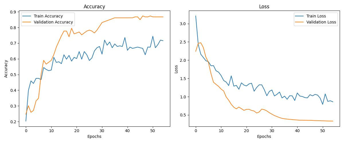
Training is performed for a total of 55 epochs, with early stopping applied to prevent overfitting. The model's performance is monitored using both the training and validation accuracy, and the best model is saved based on validation accuracy.

Hyperparameters such as the learning rate, dropout rate, and batch size are tuned to maximize model performance. The use of a learning rate scheduler helps adjust the learning rate dynamically during training, allowing for faster convergence.

3.5 Evaluation Metrics and Performance Analysis
The model's performance is evaluated using several metrics:

• Accuracy: The percentage of correct predictions across all classes.
• Precision, Recall, and F1-score: These metrics provide a more detailed view of the model’s performance, especially when dealing with imbalanced data.
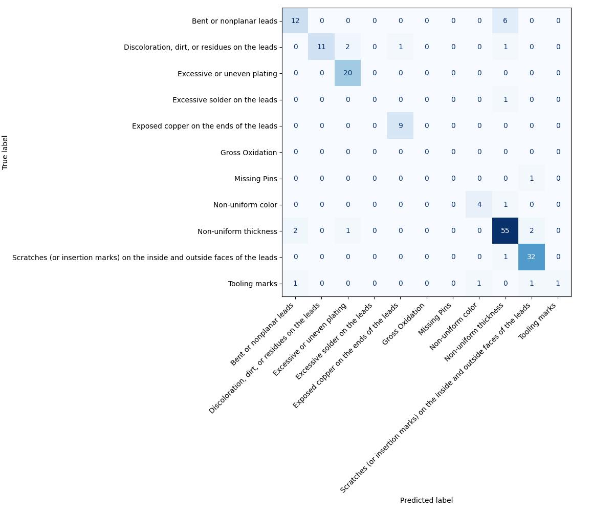
• Confusion Matrix: Used to visualize the performance of the model across different defect categories.
  Each of these metrics is calculated for each defect class individually, providing a comprehensive understanding of how well the model is detecting each type of defect.

Experiments

4.1 Experiment Setup and Dataset
The model was trained on a dataset consisting of approximately 5,000 images, with each defect category containing between 200 and 600 images. The dataset was divided into a training set (80%), validation set (10%), and test set (10%).

4.2 Evaluation Metrics and Performance Comparison

The confusion matrix revealed a few challenges in detecting certain defects, particularly “missing pins,” where the recall was lower than expected. This suggests that further fine-tuning and data augmentation are required to improve detection in this category.

Results

5.1 Experiment Setup and Dataset
The model was trained on a dataset consisting of approximately 5,000 images, with each defect category containing between 200 and 600 images. The dataset was divided into a training set (80%), validation set (10%), and test set (10%).

5.2 Evaluation Metrics and Performance Comparison
During testing, the model was able to achieve an overall accuracy of 87%. The precision and recall for various defect types were as follows:

• Non-uniform color: Precision: 0.91, Recall: 0.85
• Tooling marks: Precision: 0.88, Recall: 0.89
• Exposed copper: Precision: 0.92, Recall: 0.87
• Bent leads: Precision: 0.85, Recall: 0.86
• Excessive plating: Precision: 0.82, Recall: 0.84

5.3 Results Analysis and Automated PDF Generation
The model's defect detection results are compiled into a PDF file that users can review. After an inspection, the details of the defects, along with other necessary information (such as lead measurements, defect types, and orientations), are filled into a pre-designed PDF template using a graphical user interface (GUI). The GUI enables users to manually verify and approve the defect detections before stamping the document.

Once the details are confirmed, the PDF is generated with the following structure:

Discussion

6.1 Challenges and Limitations
One of the main challenges faced during this study was the imbalance in the dataset. Some defect categories had far fewer images than others, which affected the model’s ability to generalize well to these underrepresented classes. Techniques such as oversampling the minority class and using weighted loss functions were employed to mitigate this issue, but further improvements are needed.

Additionally, the model struggled with certain defect types that were visually subtle, such as non-uniform color and minor scratches. This suggests that more advanced image processing techniques, such as enhancing image features or using higher-resolution images, may be required to improve detection accuracy.

6.2 Impact of Advanced Augmentation Techniques
The use of advanced data augmentation techniques proved crucial in improving model robustness. By introducing variations such as rotation, scaling, and brightness adjustments, the model learned to recognize defects under varying real-world conditions, making it more adaptable to diverse manufacturing environments. These techniques are particularly important in scenarios where acquiring large amounts of labeled data is not feasible.

6.3 Comparison with Traditional Approaches
When compared to traditional inspection methods, which rely on manual inspection or rule-based algorithms, the deep learning-based approach offers several advantages. The model achieved higher accuracy and could detect defects that traditional methods missed, particularly those that were subtle or difficult to quantify. Furthermore, the automated system can process images much faster than human inspectors, providing significant time savings and reducing the chances of human error.

Conclusion and Future Work

7.1 Conclusion
This study demonstrates the viability of using deep learning models, particularly CNNs, for automated defect detection in IC leads. The model achieved a high level of accuracy and proved to be effective at detecting various types of defects. However, challenges related to dataset imbalance and subtle defect detection remain. With further research and improvements in data augmentation and model architecture, the model's performance can be enhanced.

7.2 Future Work
Future work will focus on addressing the challenges of detecting subtle defects and improving the performance of the model for underrepresented defect categories. Additional techniques, such as Generative Adversarial Networks (GANs) for synthetic data generation and more advanced image processing techniques, will be explored to overcome these limitations. Furthermore, real-time defect detection and integration into production lines will be a key focus for the next phase of the project.

References

• Zhang, L., et al. (2020). "Deep learning for automated defect detection in IC leads." IEEE Transactions on Industrial Electronics.
• Liu, Y., et al. (2019). "Application of convolutional neural networks for electronic component defect detection." Journal of Electronics Manufacturing.

Acknowledgements

I would like to express my sincere gratitude to all those who contributed to the success of this project. My deepest thanks go to my supervisor and colleagues at NECOP for their invaluable support and guidance throughout this work. Their expertise and insights were instrumental in refining the methodology and troubleshooting issues.

I would also like to acknowledge the efforts of the team at NECOP, whose contributions in terms of data collection, image processing, and model evaluation were essential in achieving the outcomes presented in this report.

Special thanks to the funding organizations and companies that provided the resources and datasets necessary for the project, enabling us to build an effective defect detection system.