Abstract

In this article we will explore the Polars library, a data manipulation framework designed to address limitations of traditional tools like pandas. We dive into the core philosophy of Polars, emphasizing its columnar, immutable, and lazy evaluation principles, which contribute to its speed and scalability. Highlighting the key features such as lightning-fast query engine, support for complex data types, and integration with Python Ecosystems. We also look into a detailed overview of the important functions of LazyAPI. Furthermore, a comparison with Pandas sheds light on Polars' advantages in performance, scalability, and memory usage, while also addressing its current limitations and learning curve. By examining its pros and cons, this article aims to equip readers with the knowledge to evaluate Polars as a viable alternative for their data manipulation needs, particularly in scenarios requiring high efficiency and scalability.

Introduction

For Data Science, Python has been the go-to language due to its versatility and extensive ecosystem of user-friendly libraries like Numpy, pandas, and Dask. Data Analysis and Manipulation play an important role in extracting insights and making informed decisions. However, as datasets grow in size and complexity, the demand for high-performance solutions becomes increasingly important.

Handling large datasets efficiently and quickly requires tools that provide fast computations and optimized operations. This is where Polars comes into the picture, generating a significant amount of buzz lately.

Polars is a powerful, high-performance, open-source DataFrame library designed for manipulating structured data and provides fast and efficient data processing capabilities. Inspired by the ubiquitous pandas library, Polars not only matches its functionality but elevates it by offering a seamless experience for working on large datasets that might not fit into the memory. The core of this library is written in Rust, and available for Python, R, and NodeJS.

Getting to know Polars

Polars was developed by Richie Vink in 2020. It combines the flexibility and user-friendliness of Python and the speed and high scalability of Rust, making it an intriguing choice for a wide range of data processing tasks. Its lightning-fast speed is what makes it stand out. The core of Polars is built in Rust, a low-level language that operates with no external dependencies and offers high memory efficiency. This combination allows Polars to achieve performance on par with C or C++. Furthermore, Polars ensures that all available CPU cores are used in parallel, enabling efficient data processing, while also supporting large datasets without requiring all data to be loaded in the memory.

Another feature of the Polars Library is its extensive and intuitive API for efficient data manipulation and analysis. Its API is designed to be user-friendly and follows a method-chaining style similar to pandas. This allows you to utilize your existing knowledge and codebase while benefiting from Polars' performance enhancement. Its query engine utilizes Apache Arrow to run vectorized queries. This is yet another feature that gives Polars a performance boost.

Philosophy

The aim of Polars is to provide a swift DataFrame library that:

1. Utilizes all available CPU cores on your system.
2. Processes datasets that are much larger than the available RAM.
3. Offers a consistent and intuitive API
4. Adheres to a strict schema, requiring data types to be defined before queries.
   Polars' columnar storage model is integral to its performance, enabling efficient operations on large datasets.

Key Features

1. Speed and Performance: Designed for high performance, utilizing parallel processing and memory optimization strategies to handle large datasets much more efficiently. For instance, consider processing a dataset of financial transactions to identify potential fraud. In a typical workflow, a large dataset might be scanned for anomalies like unusually high transaction amounts or suspicious patterns. Using Polars' parallel processing, such tasks can be performed significantly faster.

2. Data Manipulation Capabilities: Offers a robust set of tools for data manipulation, including key operations like filtering, sorting, grouping, joining and aggregating data. Although Polars may not have the same extensive functionality as pandas due to its relative novelty, it supports around 80% of the typical operations available in pandas.

3. Expressive Syntax: Polars uses a clear and user-friendly syntax, making it simple to learn and work with. It enables users to transition easily.

Installation

To install Polars Library in Python, you can use pip, Polars supports Python version 3.7 and above. Here's how to do it:

• Basic Installation for the standard version of Polars

pip install polars

• Installation with feature enhancements : If you need any additional features like parquet or CSV support, you can install Polars with optional dependencies.

pip install polars[all]

Polars DataFrames

Using Polars you can create a DataFrame in a few lines of code. To create a DataFrame, you use the pl.DataFrame() constructor. This constructor supports two-dimensional data in multiple formats. Here's an example to demonstrate how to create a DataFrame, from a dictionary of random data about student heights and weights.

import polars as pl
df = pl.DataFrame(
    {
        "name": ["Liam Johnson", "Eva Smith", "Aron Davis", "Isabella Donovan"],
        "weight": [72.5, 57.9, 83.1, 53.6],  # (kg)
        "height": [1.77, 1.56, 1.75, 1.48],  # (m)
        "age":[21,18,22,19] 
    }
)
print(df)

shape: (4, 4)
┌──────────────────┬────────┬────────┬─────┐
│ name             ┆ weight ┆ height ┆ age │
│ ---              ┆ ---    ┆ ---    ┆ --- │
│ str              ┆ f64    ┆ f64    ┆ i64 │
╞══════════════════╪════════╪════════╪═════╡
│ Liam Johnson     ┆ 72.5   ┆ 1.77   ┆ 21  │
│ Eva Smith        ┆ 57.9   ┆ 1.56   ┆ 18  │
│ Aron Davis       ┆ 83.1   ┆ 1.75   ┆ 22  │
│ Isabella Donovan ┆ 53.6   ┆ 1.48   ┆ 19  │
└──────────────────┴────────┴────────┴─────┘

In the above example we first import Polars and define the data using dictionary with entries name, weight and height. These then become the 3 columns of the Polars DataFrame.

Here’s how you can create a DataFrame of a csv file using the read_csv() method.

data=pl.read_csv("dataset.csv")
data.head()

Polars DataFrames are equipped with numerous methods and attributes for exploring data. Let's see some of them in action on the DataFrame we created earlier.

• schema: Dictionaries that tell you the data type of each column.

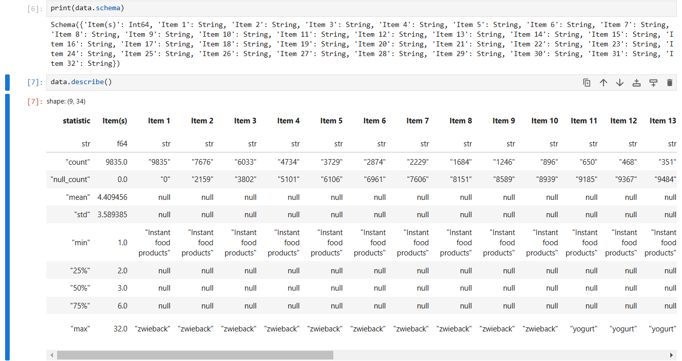
print(data.schema)

• head(): Gives you a preview of the first 5 rows of the DataFrame. You can pass any integer to the .head() method, depending on the number of rows you want to see, the default number is 5. Polars also has a .tail() method that allows you to view the bottom 5 rows.

• describe(): Gives you the statistical summary of each column in the DataFrame. It helps in quickly
  understanding the data's distribution and includes the following details:
  -Mean: The average value of the column.
  -Standard Deviation: A measure of the amount of variation in the data.
  -Minimum Value: The smallest value in the column.
  -Maximum Value: The largest value in the column.
  -Median: The middle value when the column's data is sorted.
  -Count: The total number of non-null entries in the column.
  -Data Type: The data type of the column.

data.describe()

Expressions and Contexts

Expressions and Contexts are the core components of Polars as they provide a modular and expressive way of expressing data transformations.

bmi_ex= pl.col("weight")/(pl.col("height")**2) #expression
print(bmi_ex)

[(col("weight")) / (col("height").pow([dyn int: 2]))]

An expression in Polars Expressions are instructions to the Polars query engine. Instead of directly applying an operation to data, Polars creates a plan (an expression) that will be executed later, which is a part of its lazy evaluation model, allowing optimization. Expressions can include mathematical operations, comparisons, aggregations, and string manipulations.

Contexts are the environment in which expressions are evaluated. They are the fundamental action that you want to perform on your data. Contexts determine how the expressions are evaluated and executed. Polars has 3 main contexts:

1. Select Context:

The select Context applies expressions over columns. The context select may produce new columns that are aggregations, combinations of other columns, or literals.
The with_columns Context is very similar to the Select Context. The main difference between the two is that with_columns creates a new DataFrame that contains columns from the original DataFrame and the new columns according to its input expressions, whereas the context select only incudes the columns selected by its input expressions.

#select
select_con = df.select(
    bmi=bmi_ex,
    avg_bmi=bmi_ex.mean(),
    ideal_max_bmi=25,
)
print(select_con)

shape: (4, 3)
┌───────────┬──────────┬───────────────┐
│ bmi       ┆ avg_bmi  ┆ ideal_max_bmi │
│ ---       ┆ ---      ┆ ---           │
│ f64       ┆ f64      ┆ i32           │
╞═══════════╪══════════╪═══════════════╡
│ 23.141498 ┆ 24.63463 ┆ 25            │
│ 23.791913 ┆ 24.63463 ┆ 25            │
│ 27.134694 ┆ 24.63463 ┆ 25            │
│ 24.470416 ┆ 24.63463 ┆ 25            │
└───────────┴──────────┴───────────────┘

with_columns

#with_columns
with_con = df.with_columns(
    bmi=bmi_ex,
    avg_bmi=bmi_ex.mean(),
    ideal_max_bmi=25,
)
print(with_con)

shape: (4, 7)
┌──────────────────┬────────┬────────┬─────┬───────────┬──────────┬───────────────┐
│ name             ┆ weight ┆ height ┆ age ┆ bmi       ┆ avg_bmi  ┆ ideal_max_bmi │
│ ---              ┆ ---    ┆ ---    ┆ --- ┆ ---       ┆ ---      ┆ ---           │
│ str              ┆ f64    ┆ f64    ┆ i64 ┆ f64       ┆ f64      ┆ i32           │
╞══════════════════╪════════╪════════╪═════╪═══════════╪══════════╪═══════════════╡
│ Liam Johnson     ┆ 72.5   ┆ 1.77   ┆ 21  ┆ 23.141498 ┆ 24.63463 ┆ 25            │
│ Eva Smith        ┆ 57.9   ┆ 1.56   ┆ 18  ┆ 23.791913 ┆ 24.63463 ┆ 25            │
│ Aron Davis       ┆ 83.1   ┆ 1.75   ┆ 22  ┆ 27.134694 ┆ 24.63463 ┆ 25            │
│ Isabella Donovan ┆ 53.6   ┆ 1.48   ┆ 19  ┆ 24.470416 ┆ 24.63463 ┆ 25            │
└──────────────────┴────────┴────────┴─────┴───────────┴──────────┴───────────────┘

2. Filter Context:

The Filter Context filters the rows of a DataFrame based on one or more expressions that evaluate to the Boolean data type.

#filter
filter_con = df.filter(
    pl.col("age")>20
)
print(filter_con)

shape: (2, 4)
┌──────────────┬────────┬────────┬─────┐
│ name         ┆ weight ┆ height ┆ age │
│ ---          ┆ ---    ┆ ---    ┆ --- │
│ str          ┆ f64    ┆ f64    ┆ i64 │
╞══════════════╪════════╪════════╪═════╡
│ Liam Johnson ┆ 72.5   ┆ 1.77   ┆ 21  │
│ Aron Davis   ┆ 83.1   ┆ 1.75   ┆ 22  │
└──────────────┴────────┴────────┴─────┘

3. GroupBy and Aggregation Context:

In the GroupBy Context the rows are grouped according to the unique values of the expression. This is useful for computing summary statistics within subgroups of your data.

#Group_by
gb_con = df.group_by(
        (pl.col("age") < 20).alias("Old?"),
        (pl.col("height") < 1.7).alias("Short?"),   
).agg(pl.col("name"))

print(gb_con)

shape: (2, 3)
┌───────┬────────┬─────────────────────────────────┐
│ Old?  ┆ Short? ┆ name                            │
│ ---   ┆ ---    ┆ ---                             │
│ bool  ┆ bool   ┆ list[str]                       │
╞═══════╪════════╪═════════════════════════════════╡
│ false ┆ false  ┆ ["Liam Johnson", "Aron Davis"]  │
│ true  ┆ true   ┆ ["Eva Smith", "Isabella Donova… │
└───────┴────────┴─────────────────────────────────┘

Since expressions in Polars are evaluated lazily, the library can optimize and simplify your expression before executing the data transformation it represents. Within a context, separate expressions can be processed in parallel, and Polars also leverages parallel execution when expanding expressions.

Lazy API

The Lazy API is a powerful feature that enables you to write and execute complex data transformation pipelines efficiently. With this API, you can specify a sequence of operations without immediately running them, until the .collect() method is called. This deferred execution allows Polars to optimize queries before execution and perform memory-efficient queries on datasets that don't fit into memory.

df_lazy=pl.LazyFrame(df)
df_lazy

naive plan: (run LazyFrame.explain(optimized=True) to see the optimized plan)
DF ["name", "weight", "height", "age"]; PROJECT */4 COLUMNS

The core object within the lazy API is the LazyFrame. When working with LazyFrame, operations such as filtering, selecting, joining or aggregating data do not execute immediately. Instead, it builds a query plan that describes the transformations that are to be applied to the data. The plan is only executed when the .collect() is called, ensuring all operations are processed in a single pass.

lazy_query = (
     df_lazy
     .with_columns(
         (pl.col("weight") / pl.col("height")**2).alias("bmi")
    )
  )
res=lazy_query.collect()
print(res)

shape: (4, 5)
┌──────────────────┬────────┬────────┬─────┬───────────┐
│ name             ┆ weight ┆ height ┆ age ┆ bmi       │
│ ---              ┆ ---    ┆ ---    ┆ --- ┆ ---       │
│ str              ┆ f64    ┆ f64    ┆ i64 ┆ f64       │
╞══════════════════╪════════╪════════╪═════╪═══════════╡
│ Liam Johnson     ┆ 72.5   ┆ 1.77   ┆ 21  ┆ 23.141498 │
│ Eva Smith        ┆ 57.9   ┆ 1.56   ┆ 18  ┆ 23.791913 │
│ Aron Davis       ┆ 83.1   ┆ 1.75   ┆ 22  ┆ 27.134694 │
│ Isabella Donovan ┆ 53.6   ┆ 1.48   ┆ 19  ┆ 24.470416 │
└──────────────────┴────────┴────────┴─────┴───────────┘

In the above example, the BMI calculation is achieved by dividing the values in the weight column by the square of the corresponding values in the height column. This calculation is expressed using Polars' column expressions, where pl.col("weight") refers to the weight column, and pl.col("height") refers to the height column. The expression (pl.col("weight") / pl.col("height")**2) performs element-wise operations on these columns to compute BMI for each row in the dataset.

Common Data Manipulation Functions with Polars

• sort() method to sort a DataFrame based on one or more columns.

• drop_nulls() method allows you to drop rows that contain any missing values.

• join() method provides flexible options for joining and combining DataFrames, allowing you to merge and concatenate data from different sources.

Polars vs Pandas

Pandas had been the go-to analysis tool in the python ecosystem for over a decade. It is known for its flexibility and ease of use. It provides a very user-friendly interface for working with data. Even though it has grown and evolved over time, as a result some of its core parts might be showing their age. Pandas is inherently single-threaded and processes data row by row or column by column, making it less efficient when working with very large datasets. Moreover, Pandas stores data un memory, which can lead to performance bottlenecks.

Polars brings a new approach to working with data. It has specifically been designed to work with large datasets efficiently. With the above discussed Lazy strategy and the parallel execution capabilities, it excels at processing huge amounts of data. Polars minimizes memory usage through its efficient data representation.

From a usability perspective, Pandas is widely known and has an extensive ecosystem of libraries built around it. Its familiar syntax makes it easier to integrate into existing workflows. Polars, while less established, is gaining traction due to its speed and scalability. It has a similar syntax to Pandas, which makes it accessible for new users.

On the other hand in terms of performance, Polars often outperforms pandas when handling large datasets or computationally expensive operations. While pandas can struggle with memory usage and processing time as the data increases, Polars excels by leveraging parallelism. However, for smaller datasets, pandas remains a convenient choice.

Here is an example demonstrating the execution speeds of Polars and Pandas, here we'll create a dataset with 100 million rows and a single column of random integers. Then, we'll sort this dataset in ascending order, comparing the time taken by both the libraries to sort the data.

import pandas as pd
import polars as pl
import numpy as np
import time

# Create a large DataFrame for Pandas (100 million rows)
n = 100_000_000
df_pandas = pd.DataFrame({
    'col1': np.random.randint(0, 1000, size=n)
})

# Create a large DataFrame for Polars (100 million rows)
df_polars = pl.DataFrame({
    'col1': np.random.randint(0, 1000, size=n)
})

# Timing the sort operation for Pandas
start_time = time.time()
df_pandas_sorted = df_pandas.sort_values('col1')
pandas_time = time.time() - start_time

# Timing the sort operation for Polars
start_time = time.time()
df_polars_sorted = df_polars.sort('col1')
polars_time = time.time() - start_time

# Output the time taken for each operation
print(f"Pandas sort time: {pandas_time:.6f} seconds")
print(f"Polars sort time: {polars_time:.6f} seconds")

Pandas sort time: 30.629181 seconds
Polars sort time: 1.425679 seconds

We can see that Polars is around 10 times faster than Pandas for sorting a 100 million-row dataset. This demonstrates Polars' efficiency with large data sizes due to its parallel processing and optimized memory usage.

Integration

Polars supports reading data from a wide range of popular data sources. This means, for many use cases, Polars can replace whatever data processing library you are currently working with. You will now explore examples that demonstrate Polars' versatility in handling various data sources and its comparability with different libraries.

Polars can also handle data sources like JSON, Parquet, Avro and Excel, including some databases like MySQL, PostgreSQL and Oracle Database. Here is an example:

import polars as pl

#Create a DataFrame
data = pl.DataFrame({
    "A": [1, 2, 3, 4, 5],
     "B": [6, 7, 8, 9, 10],
 })

data.write_csv("data.csv")
data.write_ndjson("data.json")
data.write_parquet("data.parquet")

Polars delivers a robust collection of tools for handling widely used data sources. Up next, you'll discover how Polars works effortlessly with other Python libraries, allowing it to fit smoothly into existing projects with little hassle.

Polars integrates seamlessly with existing Python libraries. This is a crucial feature because it allows you to drop Polars into existing code without having to change your dependencies or do a big refactor. Once you import NumPy, Pandas, and Polars, you can create identical datasets using each of the three libraries. By working with Polars DataFrame, Pandas DataFrame, and NumPy arrays, you can test how well these libraries interact with one another. For instance, you can easily convert a Pandas DataFrame and a NumPy array into Polars DataFrames using the following functions:

polars_data = pl.DataFrame({
     "A": [1, 2, 3, 4, 5],
     "B": [6, 7, 8, 9, 10]
 })

pandas_data = pd.DataFrame({
     "A": [1, 2, 3, 4, 5],
     "B": [6, 7, 8, 9, 10]
 })

numpy_data = np.array([
     [1, 2, 3, 4, 5],
     [6, 7, 8, 9, 10]
 ]).T
pl.from_pandas(pandas_data)
pl.from_numpy(numpy_data, schema={"A": pl.Int64, "B": pl.Int64})

pl.from_pandas() converts your pandas DataFrame to a Polars DataFrame. Similarly, pl.from_numpy() converts your NumPy array to a Polars DataFrame. If you want your columns to have the right data types and names, then you should specify the schema argument when calling pl.from_numpy().

Pros and Cons

Real-Life Implementations

1. E-Commerce: Analyzing sales data to calculate key metrics like total revenue or identifying the best-performing products. Here's an example where we calculate the total revenue per product category:

import polars as pl

# Correct the dataset variable name and structure
data1 = {
    "category": ["Electronics", "Clothing", "Clothing", "Electronics"],
    "sales": [1000, 1500, 2000, 3000]
}

# Create a DataFrame
df1 = pl.DataFrame(data1)

# Perform grouping and aggregation
result = df1.group_by("category").agg(pl.sum("sales").alias("total_revenue"))

# Print the result
print(result)

shape: (2, 2)
┌─────────────┬───────────────┐
│ category    ┆ total_revenue │
│ ---         ┆ ---           │
│ str         ┆ i64           │
╞═════════════╪═══════════════╡
│ Electronics ┆ 4000          │
│ Clothing    ┆ 3500          │
└─────────────┴───────────────┘

2. Finance: Performing calculations like calculating interest rates or analysis on investment portfolios. I the following example we calculate compound interest by generating a DataFrame:

#Compound interest
data = {
    "principal": [1000, 1500],
    "rate": [0.05, 0.04],
    "time": [5, 10]
}
df = pl.DataFrame(data)
df = df.with_columns((pl.col("principal") * (1 + pl.col("rate")) ** pl.col("time")).alias("future_value"))
print(df)

shape: (2, 4)
┌───────────┬──────┬──────┬──────────────┐
│ principal ┆ rate ┆ time ┆ future_value │
│ ---       ┆ ---  ┆ ---  ┆ ---          │
│ i64       ┆ f64  ┆ i64  ┆ f64          │
╞═══════════╪══════╪══════╪══════════════╡
│ 1000      ┆ 0.05 ┆ 5    ┆ 1276.281563  │
│ 1500      ┆ 0.04 ┆ 10   ┆ 2220.366427  │
└───────────┴──────┴──────┴──────────────┘

3. Healthcare: Analyzing patient data for trends or calculating BMI.

Conclusion

In conclusion, the Polars library offers a modern alternative with high performance to traditional data manipulation tools, especially for larger datasets. Its design is optimized for modern hardware and efficient memory usage, which allows faster processing and scalability. It also simplifies method chaining and enhances usability. However, it is still evolving and some users may encounter some limitations like the lack of built-in plotting and a smaller ecosystem when compared to pandas. Despite this, Polars prove to be a promising tool for data processing and manipulation tasks. As the library continues to evolve and mature, it has the potential to become a key player in the data science and analysis industry.
Thank You!