Predicting Gold Prices with LSTM-CNN: A Simple Explanation

Gold price forecasting is tricky because prices are very unpredictable. To tackle this, I worked on a project inspired by a paper titled "Gold Price Forecast Based on LSTM-CNN Model." In this project, I used a mix of deep learning and statistical models to try and predict daily gold prices.
Let me break it down for you!

What Did I Do?

I started by collecting historical gold price data from the World Gold Council. The data had daily gold prices spanning many years. My goal was to build models that could predict future gold prices accurately.
First, I cleaned the data by handling missing values and scaling it for better performance in machine learning models. I then split the data into training and testing sets, ensuring that my models had unseen data for evaluation. After preprocessing, I explored various prediction methods. These included traditional models like ARIMA and SVR, as well as deep learning models like LSTM and CNN. Each model had its strengths and weaknesses, which I analyzed in detail.
Finally, I combined architectures like LSTM and CNN, and even added an attention mechanism to boost accuracy. The performance of each model was carefully evaluated using metrics like MSE and MAE to find the best approach.

The Data

The dataset came from the World Gold Council. It included daily gold prices over many years. Before jumping into modeling, I:

• Fixed missing values.
• Scaled the data to make it suitable for machine learning.
• Split it into training and testing sets.

# Reading the dataset
data_csv = "./dataset.csv"
df = pd.read_csv(data_csv)
df.head()

# Verifying null values and deleting name from dataset
null_columns = df.columns[df.isnull().any()]

# Drop the lines with null values
df = df.dropna()

# Transforming the dataset to ln scale
df = np.log(df["Open"].values)

timesteps = 7 
split_ratio = 0.8  

arima_data = df.copy() 
df_reshaped = df.reshape(-1, 1)  

features = []
target = []
for i in range(timesteps, len(df_reshaped)):
    features.append(df_reshaped[i - timesteps:i])
    target.append(df_reshaped[i])

features = np.array(features)
target = np.array(target)

split_index = int(len(features) * split_ratio)
train_features, test_features = features[:split_index], features[split_index:]
train_labels, test_labels = target[:split_index], target[split_index:]

scaler = MinMaxScaler(feature_range=(0, 1))
train_features_scaled = scaler.fit_transform(train_features.reshape(-1, train_features.shape[-1])).reshape(train_features.shape)
test_features_scaled = scaler.transform(test_features.reshape(-1, test_features.shape[-1])).reshape(test_features.shape)
train_labels_scaled = scaler.fit_transform(train_labels)
test_labels_scaled = scaler.transform(test_labels)

train_arima = arima_data[:int(len(arima_data) * split_ratio)]
test_arima = arima_data[int(len(arima_data) * split_ratio):]

Models I Tried

Here are the models I used, what they do, and how they performed:

Support Vector Regression (SVR)

SVR is a traditional machine learning method that works well for smaller datasets and tries to find relationships by transforming the input features into higher dimensions. However, it struggles with very noisy and large datasets like ours. SVR uses kernels (like RBF) to handle non-linear relationships, making it flexible but computationally expensive for large-scale data.

svr_model = SVR(kernel='rbf', C=100, gamma=0.1, epsilon=0.01)
svr_model.fit(train_features_scaled.reshape(train_features_scaled.shape[0], -1), train_labels_scaled.flatten())

svr_predictions = svr_model.predict(test_features_scaled.reshape(test_features_scaled.shape[0], -1))
svr_predictions_original = scaler.inverse_transform(svr_predictions.reshape(-1, 1)).flatten()

svr_mae = mean_absolute_error(test_labels, svr_predictions_original)
svr_mse = mean_squared_error(test_labels, svr_predictions_original)

Results
MAE: 0.0050556912203048865
MSE: 4.0876520287871014e-05

ARIMA

ARIMA is a statistical model that uses past values in a time series to predict future ones. It works well for datasets with clear trends or seasonality. However, ARIMA assumes linearity, so it struggles with complex, non-linear patterns like those in gold prices. It also requires careful tuning of parameters (p, d, q).

arima_order = (5, 1, 0)

arima_model = ARIMA(train_arima, order=arima_order)
arima_model_fit = arima_model.fit()
arima_predictions = arima_model_fit.forecast(steps=len(test_arima))

arima_mae = mean_absolute_error(test_arima, arima_predictions)
arima_mse = mean_squared_error(test_arima, arima_predictions)

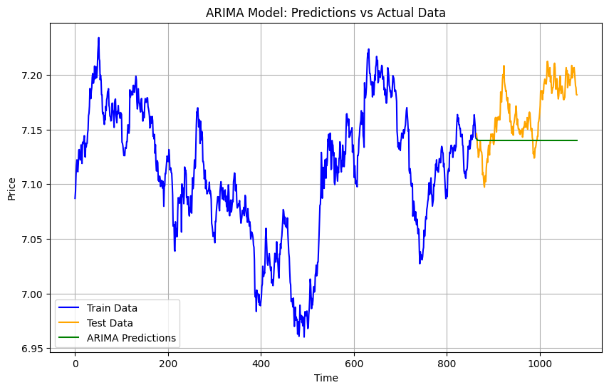
Results
MAE: 0.03105009307128872
MSE: 0.0014014216632501988

LSTM

LSTM is a type of recurrent neural network (RNN) designed to learn sequences and long-term dependencies. This makes it perfect for time series data like gold prices. It uses memory cells to retain information over time, which helps it predict future trends more effectively than traditional models.

model_lstm = Sequential([
    LSTM(50, activation='relu', input_shape=(train_features_scaled.shape[1], train_features_scaled.shape[2])),
    Dense(1)
])

model_lstm.compile(optimizer=Adam(learning_rate=0.001), loss='mean_squared_error')
model_lstm.fit(train_features_scaled, train_labels_scaled, epochs=100, batch_size=32, verbose=1)
lstm_predictions = model_lstm.predict(test_features_scaled).flatten()
lstm_predictions_original = scaler.inverse_transform(lstm_predictions.reshape(-1, 1)).flatten()

lstm_mae = mean_absolute_error(test_labels, lstm_predictions_original)
lstm_mse = mean_squared_error(test_labels, lstm_predictions_original)

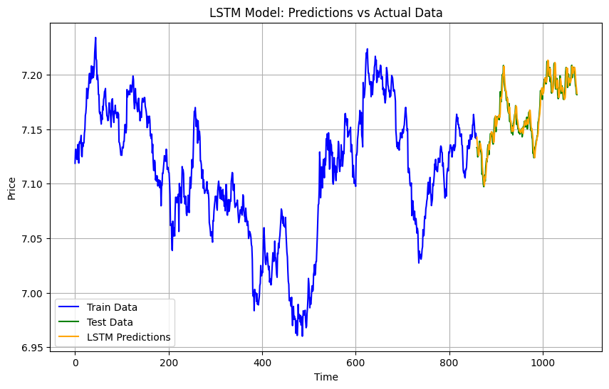
Results
MAE: 0.005403199717494776
MSE: 4.599026156625835e-05

CNN

CNN is primarily used for feature extraction. It processes data by applying convolutional filters that capture important patterns. While CNNs excel at image and spatial data, they can also identify relationships in time series data. This model helped identify localized patterns in the gold price data.

model_cnn = Sequential([
    Conv1D(64, kernel_size=2, activation='relu', input_shape=(train_features_scaled.shape[1], train_features_scaled.shape[2])),
    MaxPooling1D(pool_size=2),
    Flatten(),
    Dense(50, activation='relu'),
    Dense(1)
])

model_cnn.compile(optimizer=Adam(learning_rate=0.001), loss='mean_squared_error')
model_cnn.fit(train_features_scaled, train_labels_scaled, epochs=100, batch_size=32, verbose=1)
cnn_predictions = model_cnn.predict(test_features_scaled).flatten()
cnn_predictions_original = scaler.inverse_transform(cnn_predictions.reshape(-1, 1)).flatten()

cnn_mae = mean_absolute_error(test_labels, cnn_predictions_original)
cnn_mse = mean_squared_error(test_labels, cnn_predictions_original)

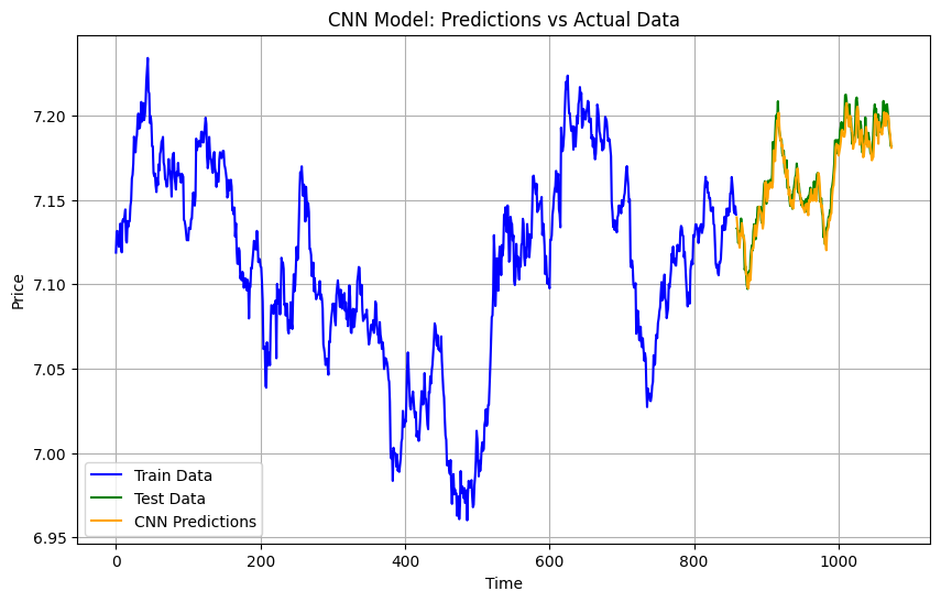
Results
MAE: 0.005676337139653184
MSE: 5.124953308100566e-05

CNN-LSTM

CNN-LSTM combines convolutional layers for feature extraction and LSTM layers for sequence learning. The CNN extracts patterns from the data, while the LSTM focuses on temporal dependencies. This hybrid model works well for data with both spatial and sequential characteristics, like gold prices.

model_cnn_lstm = Sequential([
    Conv1D(64, kernel_size=2, activation='relu', input_shape=(train_features_scaled.shape[1], train_features_scaled.shape[2])),
    MaxPooling1D(pool_size=2),
    LSTM(50, activation='relu'),
    Dense(1)
])

model_cnn_lstm.compile(optimizer=Adam(learning_rate=0.001), loss='mean_squared_error')
model_cnn_lstm.fit(train_features_scaled, train_labels_scaled, epochs=100, batch_size=32, verbose=1)
cnn_lstm_predictions = model_cnn_lstm.predict(test_features_scaled).flatten()
cnn_lstm_predictions_original = scaler.inverse_transform(cnn_lstm_predictions.reshape(-1, 1)).flatten()

cnn_lstm_mae = mean_absolute_error(test_labels, cnn_lstm_predictions_original)
cnn_lstm_mse = mean_squared_error(test_labels, cnn_lstm_predictions_original)

Results
MAE: 0.005646194209108425
MSE: 4.8779187832461365e-05

LSTM-CNN

LSTM-CNN reverses the order: it first uses LSTM layers to process sequences and then applies CNN layers to extract key features. This approach works well when temporal dependencies are more important than spatial patterns. The CNN layers add a layer of abstraction to improve accuracy.

model_lstm_cnn = Sequential([
    LSTM(50, activation='relu', return_sequences=True, input_shape=(train_features_scaled.shape[1], train_features_scaled.shape[2])),
    Conv1D(64, kernel_size=2, activation='relu'),
    MaxPooling1D(pool_size=2),
    Flatten(),
    Dense(1)
])

model_lstm_cnn.compile(optimizer=Adam(learning_rate=0.001), loss='mean_squared_error')
model_lstm_cnn.fit(train_features_scaled, train_labels_scaled, epochs=100, batch_size=32, verbose=1)
lstm_cnn_predictions = model_lstm_cnn.predict(test_features_scaled).flatten()
lstm_cnn_predictions_original = scaler.inverse_transform(lstm_cnn_predictions.reshape(-1, 1)).flatten()

lstm_cnn_mae = mean_absolute_error(test_labels, lstm_cnn_predictions_original)
lstm_cnn_mse = mean_squared_error(test_labels, lstm_cnn_predictions_original)

Results
MAE: 0.005230186119436148
MSE: 4.400704789269253e-05

LSTM-Attention-CNN

LSTM-Attention-CNN adds an attention mechanism to the hybrid model. Attention helps the model focus on the most relevant parts of the input data, boosting both temporal and spatial pattern recognition. This makes it the most accurate model for gold price forecasting in my experiments.

input_layer = tf.keras.Input(shape=(train_features_scaled.shape[1], train_features_scaled.shape[2]))
lstm_layer = LSTM(50, activation='relu', return_sequences=True)(input_layer)
attention_layer = Attention()([lstm_layer, lstm_layer])
cnn_layer = Conv1D(64, kernel_size=2, activation='relu')(attention_layer)
maxpool_layer = MaxPooling1D(pool_size=2)(cnn_layer)
flatten_layer = Flatten()(maxpool_layer)
output_layer = Dense(1)(flatten_layer)

model_lstm_attention_cnn = tf.keras.Model(inputs=input_layer, outputs=output_layer)
model_lstm_attention_cnn.compile(optimizer=Adam(learning_rate=0.001), loss='mean_squared_error')
model_lstm_attention_cnn.fit(train_features_scaled, train_labels_scaled, epochs=100, batch_size=32, verbose=1)
lstm_attention_cnn_predictions = model_lstm_attention_cnn.predict(test_features_scaled).flatten()
lstm_attention_cnn_predictions_original = scaler.inverse_transform(lstm_attention_cnn_predictions.reshape(-1, 1)).flatten()

lstm_attention_cnn_mae = mean_absolute_error(test_labels, lstm_attention_cnn_predictions_original)
lstm_attention_cnn_mse = mean_squared_error(test_labels, lstm_attention_cnn_predictions_original)

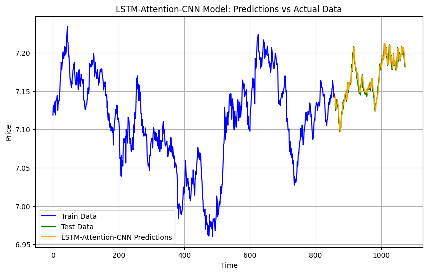
Results
MAE: 0.005221851548393977
MSE: 4.365971903156702e-05

Final Results

The LSTM-Attention-CNN model performed the best, achieving the lowest MSE and MAE values. This hybrid approach effectively captured both temporal and spatial patterns in the data. While traditional methods like ARIMA and SVR had their merits, they fell short when compared to the deep learning models.