Brain Tumor Classification System with Streamlit Web App

Abstract

This project focuses on developing a Convolutional Neural Network (CNN) to classify brain tumor MRI scans into four categories: Healthy Brain, Glioma Tumor, Meningioma Tumor, and Pituitary Tumor. The primary goal is to facilitate early diagnosis by leveraging deep learning technology to improve the accuracy of MRI image classification. Furthermore,
a Streamlit web app was developed to provide real-time classification, offering a user-friendly interface for doctors to enhance the diagnostic process.
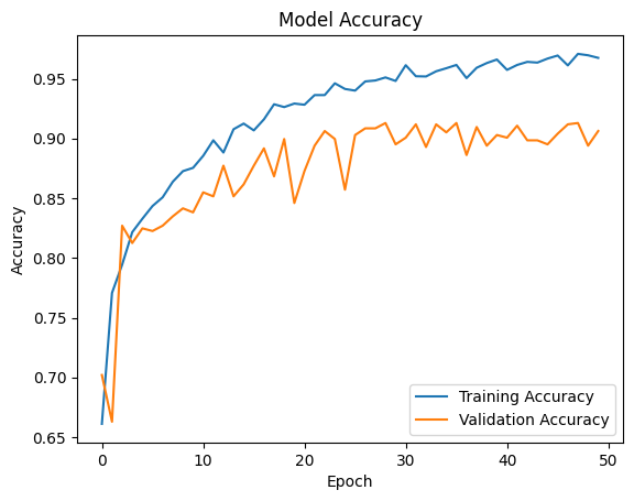
The CNN model achieved an accuracy of 97% on the training dataset and 93% on the testing dataset, demonstrating its reliability and effectiveness in distinguishing between different types of brain tumors.

Methodology

Data Collection

The dataset used for this project was sourced from Kaggle, which includes MRI scans categorized into four classes:

• Healthy Brain
• Glioma Tumor
• Meningioma Tumor
• Pituitary Tumor

The dataset consists of a diverse set of images with varying resolutions and orientations, requiring preprocessing for uniformity.

Data Preprocessing

The preprocessing steps involved the following:

• Image Loading: Images were loaded from the dataset using PIL and OpenCV.
• Resizing: All images were resized to a consistent dimension of 80x80 pixels to maintain uniformity in input data for the CNN model.
• Normalization: Each pixel value was scaled between 0 and 1 to optimize model performance.
• Splitting the Data: The dataset was split into training and testing sets with a ratio of 85% training and 15% testing to evaluate the model's performance on unseen data.

Model Development

A Convolutional Neural Network (CNN) architecture was developed to classify the MRI images. The model comprises the following layers:

• Convolutional Layers: Three convolutional layers with 32, 64, and 128 filters to extract spatial features from the MRI images.
• MaxPooling Layers: Applied after each convolutional layer to reduce the spatial dimensions and computational complexity. Fully Connected Layers: Flattening the output and passing it through dense layers, using 256 neurons for feature learning.
• Regularization: L2 regularization was applied to the convolutional and dense layers to prevent overfitting, along with Dropout for regularization.

Model Training

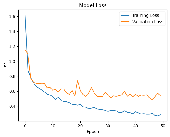
The model was trained using the Adam optimizer and Sparse Categorical Crossentropy as the loss function. The training involved 50 epochs with a batch size of 32, and a validation split of 15% of the training data was used to monitor the model's performance during training.

Model Evaluation

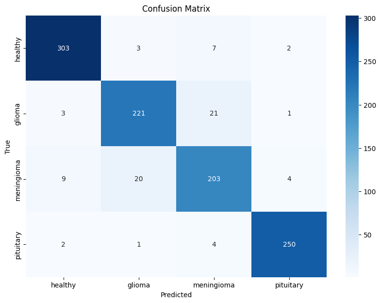
The trained CNN was evaluated on the test set, where it achieved an accuracy of 93%. Additionally, a confusion matrix and classification report were generated to analyze the model's performance across each class.

Results

The CNN model achieved 97% accuracy on the training data and 93% accuracy on the test data, proving the effectiveness of the architecture.
The confusion matrix and classification report revealed that the model performed well across all classes, with minor misclassifications between certain tumor types.

Training & Validation Loss Graph

Training & Validation Accuracy Graph

The Performance of Model on some images :-

Web Deployment

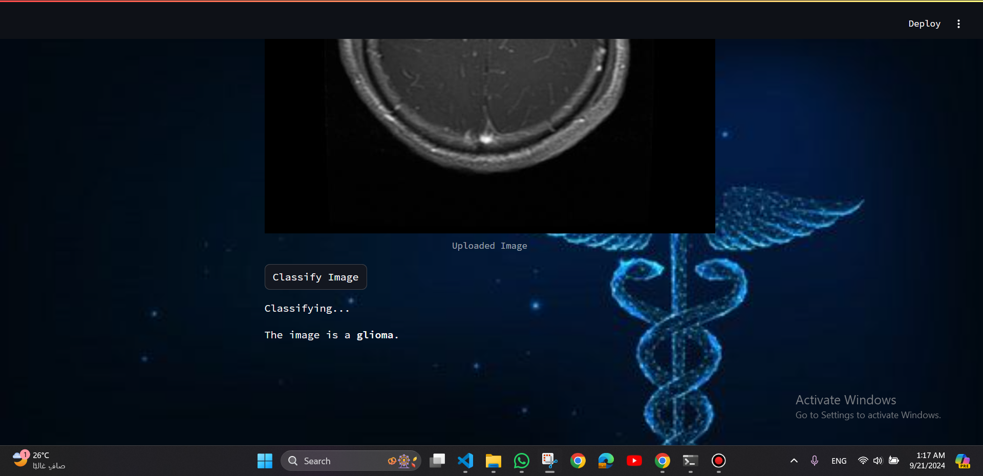
To enhance the accessibility and utility of the model, it was integrated into a Streamlit web application. The web app provides an intuitive interface for users to upload MRI images and receive real-time predictions regarding the presence of brain tumors.

Streamlit

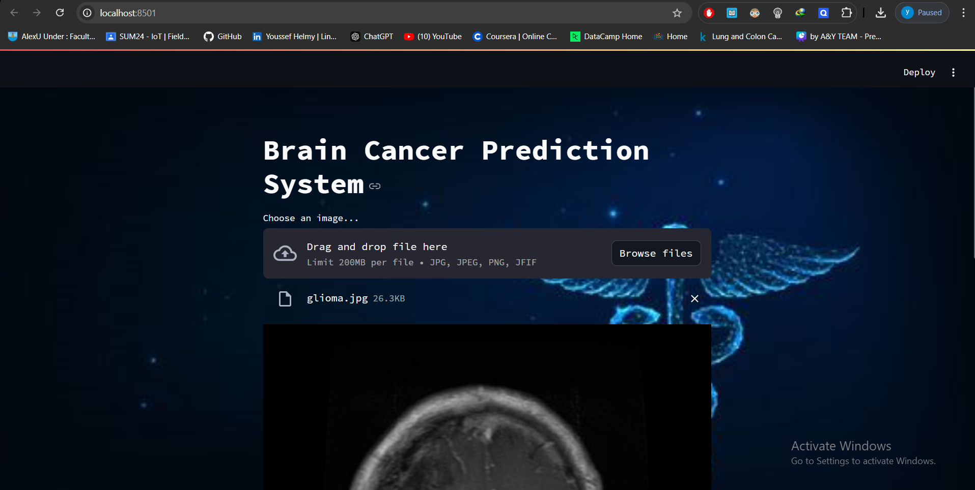
is a promising open-source Python library, which enables developers to build attractive user interfaces in no time. Streamlit is the easiest way especially for people with no front-end knowledge to put their code into a web application: No front-end (html, js, css) experience or knowledge is required.

Conclusion

This project successfully developed and deployed a deep learning-based brain tumor classification system using CNN and integrated it into a Streamlit web application for real-time classification. The model's high accuracy highlights its potential utility in aiding medical professionals in diagnosing brain tumors more efficiently.

Project Code

Brain Tumor Classification System

Import Rquired Libraries

import matplotlib.pyplot as plt
import numpy as np
import cv2
import os
import PIL
import tensorflow as tf
import pickle
import pathlib
from sklearn.model_selection import train_test_split
from tensorflow import keras
from tensorflow.keras import layers
from tensorflow.keras.regularizers import l2
from tensorflow.keras.models import Sequential

Downloading Dataset

from google.colab import files
uploaded= files.upload()
for fn in uploaded.keys():
  print('User uploaded file "{name}" with length {length} bytes'.format(
      name=fn, length=len(uploaded[fn])))

!mkdir -p ~/.kaggle && mv kaggle.json ~/.kaggle/ && chmod 600 ~/.kaggle/kaggle.json

!kaggle datasets download -d rm1000/brain-tumor-mri-scans

UnZipping brain-tumor-mri-scans images

!unzip brain-tumor-mri-scans.zip -d brain_tumor

Making a directory path for our Data

data_dir = pathlib.Path('/content/brain_tumor')

list(data_dir.glob('*/*.jpg'))[:5]

Getting The number of Images in Dataset

image_count = len(list(data_dir.glob('*/*.jpg')))
print(image_count)

listing all brain glioma Images

glioma = list(data_dir.glob('glioma/*'))
PIL.Image.open(str(glioma[0]))

listing all brain healthy Images

healthy= list(data_dir.glob('healthy/*'))
PIL.Image.open(str(healthy[0]))

listing all brain meningioma Images

meningioma= list(data_dir.glob('meningioma/*'))
PIL.Image.open(str(meningioma[0]))

listing all brain pituitary Images

pituitary= list(data_dir.glob('pituitary/*'))
PIL.Image.open(str(pituitary[0]))

Plotting The Count of each Class

# Count the number of images in each class
glioma_count = len(list(data_dir.glob('glioma/*.jpg')))
healthy_count = len(list(data_dir.glob('healthy/*.jpg')))
meningioma_count = len(list(data_dir.glob('meningioma/*.jpg')))
pituitary_count = len(list(data_dir.glob('pituitary/*.jpg')))


# Create a pie chart
labels = ['Brain Glioma', 'Healthy Brain', 'Meningioma Brain','Pituitary Brain']
sizes = [glioma_count, healthy_count,meningioma_count ,pituitary_count ]
colors = ['red', 'green', 'yellow','pink']
explode = (0.1, 0.1, 0.1,0)  # explode the 1st slice

plt.pie(sizes, explode=explode, labels=labels, colors=colors,
        autopct='%1.1f%%', shadow=True, startangle=140)

plt.axis('equal')  # Equal aspect ratio ensures that pie is drawn as a circle.

plt.title('Distribution of Brain Cancer MRI Images')
plt.show()

Making a dictionary for all lung Images

brain_images_dict = {
    'healthy': list(data_dir.glob('healthy/*')),
    'glioma': list(data_dir.glob('glioma/*')),
    'meningioma': list(data_dir.glob('meningioma/*')),
    'pituitary': list(data_dir.glob('pituitary/*')),
}

Making a dictionary for all lables

brain_labels_dict = {
    'healthy': 0,
    'glioma': 1,
    'meningioma': 2,
    'pituitary':3,

}

Separating The Features and Target and Resizing The Images

X, y = [], []
for diagnosis, images in brain_images_dict.items():
    for image in images:
        img = cv2.imread(str(image))
        resized_img = cv2.resize(img,(80,80))
        X.append(resized_img)
        y.append(brain_labels_dict[diagnosis])

X = np.array(X)
y = np.array(y)

Splitting The Data into train and test

X_train, X_test, y_train, y_test = train_test_split(X, y, test_size=0.15 , random_state=42)

Normaliztion

X_train_scaled = X_train / 255.0
X_test_scaled = X_test / 255.0

CNN Architecture

# CNN Architecture with Regularization and Dropout
num_classes = 4

model1 = Sequential([
    layers.Conv2D(32, 3, padding='same', activation='relu', kernel_regularizer=l2(0.01)),
    layers.MaxPooling2D(),

    layers.Conv2D(64, 3, padding='same', activation='relu', kernel_regularizer=l2(0.01)),
    layers.MaxPooling2D(),


    layers.Conv2D(128, 3, padding='same', activation='relu', kernel_regularizer=l2(0.01)),
    layers.MaxPooling2D(),


    layers.Flatten(),
    layers.Dense(256, activation='relu', kernel_regularizer=l2(0.01)),


    layers.Dense(num_classes, activation='softmax')
])

model1.compile(optimizer='adam', loss=tf.keras.losses.SparseCategoricalCrossentropy(), metrics=['accuracy'])

# Train the model
history = model1.fit(X_train_scaled, y_train, validation_split=0.15, batch_size=32, epochs=50)

Evaluating The Model

model1.evaluate(X_test_scaled,y_test)

Prediction of Model

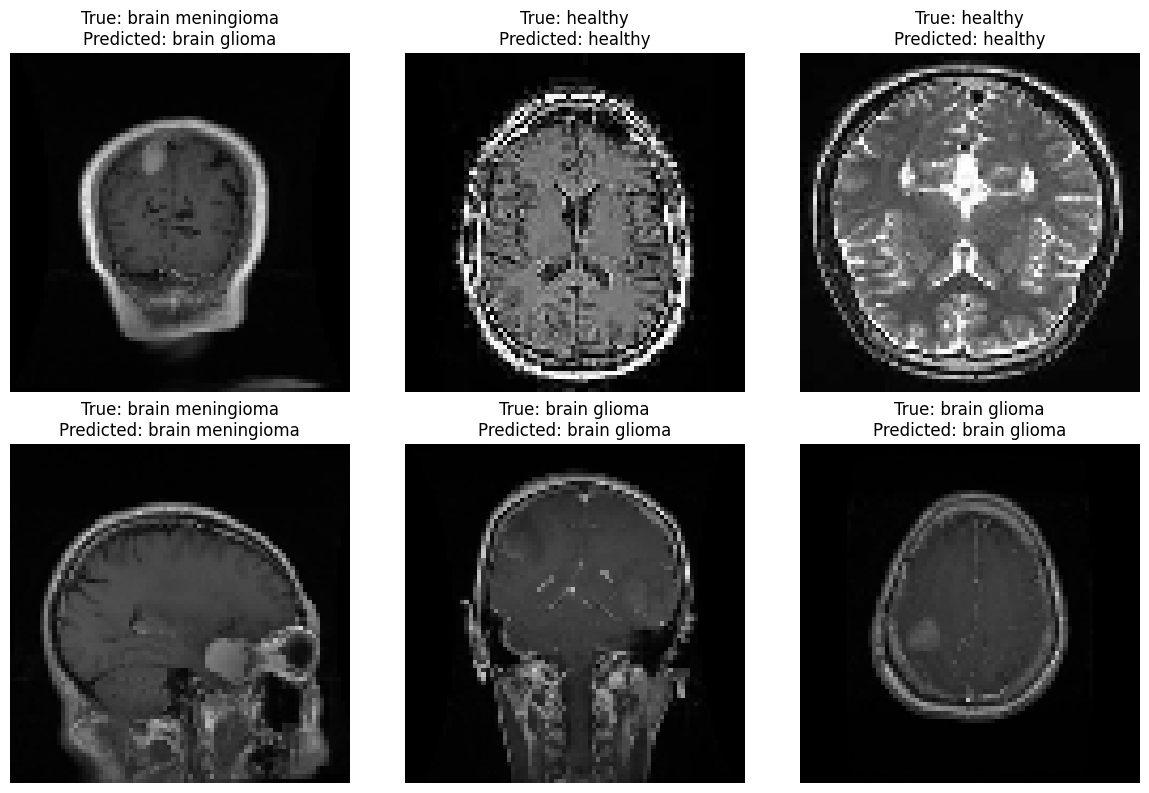
predictions = model1.predict(X_test_scaled)

plotting random images with predicted and True Class

label_to_class = {
    0: 'healthy',
    1: 'brain glioma',
    2: 'brain meningioma',
    3: 'brain pituitary',
}

# Select a random subset of images to display
num_images_to_display = 6
random_indices = np.random.choice(len(X_test), num_images_to_display, replace=False)

# Create a figure and subplots
fig, axes = plt.subplots(2, 3, figsize=(12, 8))
axes = axes.flatten()

for i, index in enumerate(random_indices):
    image = X_test[index]
    true_label = y_test[index]
    predicted_label = np.argmax(predictions[index])

    axes[i].imshow(image)
    axes[i].set_title(f"True: {label_to_class[true_label]}\nPredicted: {label_to_class[predicted_label]}")
    axes[i].axis('off')

plt.tight_layout()
plt.show()

Plot training & validation accuracy values

plt.plot(history.history['accuracy'], label='Training Accuracy')
plt.plot(history.history['val_accuracy'], label='Validation Accuracy')
plt.title('Model Accuracy')
plt.xlabel('Epoch')
plt.ylabel('Accuracy')
plt.legend(loc='lower right')
plt.show()

Plot training & validation loss values

plt.plot(history.history['loss'], label='Training Loss')
plt.plot(history.history['val_loss'], label='Validation Loss')
plt.title('Model Loss')
plt.xlabel('Epoch')
plt.ylabel('Loss')
plt.legend(loc='upper right')
plt.show()

from sklearn.metrics import classification_report

y_pred = np.argmax(predictions, axis=1)
print(classification_report(y_test, y_pred, target_names=['healthy', 'brain glioma', 'brain meningioma', 'brain pituitary']))

Confusion Matrix

import matplotlib.pyplot as plt
import numpy as np
import seaborn as sns
from sklearn.metrics import confusion_matrix

# Generate predictions for the test set
y_pred = np.argmax(model1.predict(X_test_scaled), axis=-1)

# Compute confusion matrix
cm = confusion_matrix(y_test, y_pred)

# Create a heatmap for the confusion matrix
plt.figure(figsize=(10, 7))
sns.heatmap(cm, annot=True, fmt='d', cmap='Blues',
            xticklabels=['healthy', 'glioma', 'meningioma','pituitary'],
            yticklabels=['healthy', 'glioma', 'meningioma','pituitary'])
plt.xlabel('Predicted')
plt.ylabel('True')
plt.title('Confusion Matrix')
plt.show()

Saving The Model

model1.save('Brain_Cancer_model.keras')